![]()
![]()
![]()
![]()
![]()
![]()
![]()
|
|
|
The immediately previous page dealt with
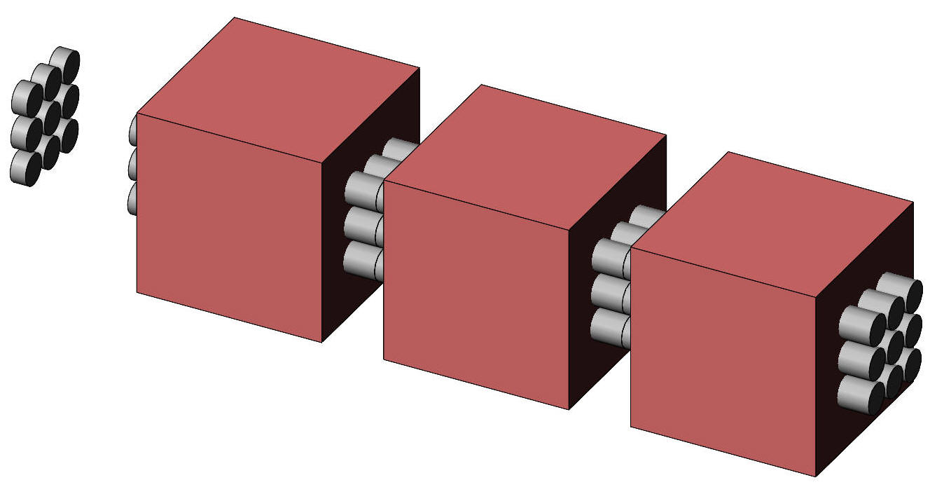
Two dependent samples. This page introduces the analysis of variance, a technique which examines the difference in mean scores for two or more groups of subjects. Anova for independent samplesA group of 9 subjects each drink a preparation containing amino acids, proteins, and peptides which the investigator expects will enhance short-term memory. The drink tastes (and smells) medicinal. A second group of 9 subjects drink a preparation that tastes medicinal but contains no active ingredients. A third group of 9 subjects drink a similar quantity of tea. All subjects then undertake a memory test. The test scores are shown in Table 1. Notice that the samples are independent – they consist of different subjects. The design is illustrated in Figure 1.
Figure 1. Representation of the one-way anova.
Table 1. Memory scores for 3 experimental groups and descriptive statistics.
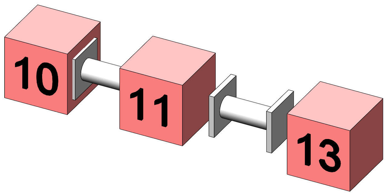
The question here is whether the protein drink improves the memory of our subjects compared to an inactive drink or to tea. The design is illustrated in Figure 2 where each cube represents the mean score of a treatment condition.
Figure 2. Representation of the means of the three treatment groups.
Profile plotAlways draw a graph to aid interpretation.
Figure 3. Profile plot of mean memory test score for Protein, Inactive, and Tea treatment groups, SE = 0.41 Inspection of the profile plot shows no overlap of the Protein treatment group error bar with either the Inactive or Tea treatments, but it the overlap between Protein and Tea treatment error bars is unclear. Since the error bars represent ±1 SE, if they do not overlap their means are separated by at least 2SE. We know that two means separated by more than 2SE could show a significant difference. We now need an appropriate statistical test to confirm this.
Testing the difference between more than two independent sample meansA possible approach to giving an answer to the question of whether one drink improves subject memory more than another drink is to construct three t-tests. One t-test compares the mean memory score of the Protein group with the Inactive; another compares Protein with Tea; and a third compares Inactive with Tea. This approach has at least three problems. The first issue is that conducting three separate significance tests raises the probability of a Type I error from α = 5% to something like 14% (§1). We could decide to conduct three separate tests using α / 3 = 1.7% as our level of significance (§2), but it would be better to have a single overall test of the significance of any differences between the means. The second issue is that, in general, each significance test would use a different SE as the estimate of the variability of the group means. The t-test comparing Protein with Inactive uses SE derived from sP and sI, comparing Protein with Tea derives SE from sP and sT, and SE for Inactive vs Tea is derived from sI and sT. Homogeneity of variance is an assumption underlying these tests, and it would be better to derive a common and better estimate of SE from all three sP, sI, and sT values together. The third issue is associated with the second. Each separate significance test uses the degrees of freedom of just two of the samples involved while ignoring the information from the third group. It would be better to have a test of significance using df of all three groups for higher test power. §1 If the probability of an event is X, the probability of the non-event is 1 – X. The probability of two non-events is (1 – X)2, the probability of three non-events is (1 – X)3, and so on. If the probability of two non-events is (1 – X)2, the probability of one or two events is 1 – (1 – X)2. If the probability of three non-events is (1 – X)3, the probability of at least one event is 1 – (1 – X)3, and so on. When X = 0.05, the probability of at least one event in 3 tries is 1 – (1 – 0.05)3 = 1 – 0.953 = 1 – 0.86 = 0.14, that is, 14.3% (before rounding). §2 Using α / c as the level of significance when there are c tests of significance is called the Bonferroni correction for a family of multiple tests.
The analysis of (mean) varianceAn ingenious approach to the question whether the protein drink improves memory compared to an inactive drink or to tea is to consider the variance that is shown by the three group means. We know that, under random sampling, the variability of a sample mean is given by its SE, s / √n. We can calculate the variability actually shown by our three sample means and check that this is within the limits suggested by random sampling. If the actual variability of the means is significantly larger than expected, we may conclude that there are significant differences between these means. There are three tasks — calculate the variance of the sample means; calculate their expected variance under random sampling; and compare these two variances. Variance shown by the sample means: The three sample means are 13, 11, and 10. Treating each mean as a single data item, their variance is 2.33 and standard deviation is 1.53. This data is laid out as Table 2.
Table 2. Sample means laid out as data items with their associated sample statistics. The standard deviation of 1.53 here corresponds to the SE of the means under the assumption they come from the same parent population whose standard deviation is given by calculating √n · SE = 3 · 1.53 = 4.58. On this evidence, the variance of the parent population is thus estimated as 4.582 = 21. Expected variance: We have three samples. From Table 1, their average standard deviation is 1.22, and this is a direct estimate of the parent population s. On this evidence, the variance of the parent population is estimated as 1.222 = 1.5. Compare observed to expected: The two estimates of the parent population variance may be compared using the F ratio, where the observed variance in the group means is divided by that expected from the variance seen within the groups. This gives a test statistic that is referred to the F distribution with two degrees of freedom, one for the observed variance and one for the expected. With p means, the df for the variance of the group means is p – 1, that is, 2 for our data. The expected variance comes from the total df of the groups; each group has df = n – 1 = 8, hence the df for the expected variance is 3 · 8 = 24 for our data. We divide the variance of the means, 21, the observed variance, by the expected variance, 1.5; for our data, F(2,24) = 21 / 1.5 = 14.0 (§3). These results are laid out in an analysis of variance summary table, and the traditional terminology applied, shown here as Table 3. Variance is termed MS, mean square. A variance is a sums of squares, SS, divided by its df. The variance shown by the group means is called between groups, and the variance shown by the samples is called within groups or within subjects but is also commonly called error and sometimes residual. To calculate the SS to complete the table (not necessary, but conventional) we multiply MS by df, hence SS(Between groups) = 21· 2 = 42, and SS(Within groups) = 1.5 · 24 = 36. Table 3. Anova summary table.
The p value for F(2,24) = 14 is <.001, highly significant. We interpret this by saying that the variance of the group means is significantly larger than might be expected by chance. This suggests that the group means therefore differ by more than might be expected by chance. The test we have made for statistical significance is called an omnibus test. It tells us in general whether the means differ, and if it is significant, (1) it implies that, at least, the largest mean is significantly larger than the smallest mean, and (2) further analysis is needed to establish exactly which means differ from which others. If the test is not significant, it tells us that there are no means which are significantly different from any others, and importantly that there is no basis for conducting any further analyses in search of any means which might differ from any others. We should check that the anova procedure has addressed the problems of undertaking separate tests of significance. Conducting three separate significance tests inflates Type I error for the experiment overall. The anova provides a single overall test of the significance of any differences between the means, so the Type I error is held at nominal α. Separate significance tests use different SEs. The anova provides a common and better estimate of SE from all three sP, sI, and sT values together, based on MS within groups or MS error. Separate significance tests use the df of just two samples. The anova provides df within groups, that is all three groups, for higher test power. Although the anova has been introduced as a method for comparing 3 or more groups, it is applicable to 2 groups and gives results identical to a t-test for two samples. §3 It may be useful to express the F ratio as a regression coefficient R when reporting the results for certain contexts. R2 is the ratio of the SS between groups to the total SS, 42 / 78 = .54, hence R is √.54 = .73. Conceptually, R is interpreted as the amount of variation in the data that is accounted for by group membership, that is, the degree to which memory scores are related to the type of drink consumed.
Pairwise and multiple comparisonsGiven the omnibus anova has shown the means differ significantly, we may now set about comparing the mean memory score of the Protein group with that of the Inactive group; the mean Protein score with the mean Tea score; and Inactive with Tea. These are called pairwise comparisons. The problem of conducting three separate significance tests returns, but at least we are under the initial protective umbrella that the overall anova provides for holding Type I error at nominal α. To begin, we derive the value of SE we need in order to test the difference between any two means of our groups. MS within groups is our estimate of the population variance, being 1.5, and √MS is the estimate of the population s, being 1.22. The estimate of the SE of a mean is s / √n, being 0.41, and the estimate of the SE of the difference between two independent means, SEdiff, is √(SE2 + SE2), which is √2SE2, being 0.58. The t-test for the difference between the means of the Protein group and the Inactive group is thus (13 – 11) / 0.58 = 3.46 with df = 24, giving p = .002 and a significant result. The degrees of freedom are those associated with SEdiff and hence are those for MS(Within groups). The critical value of t at α = .05 and df = 24 is 2.06. The t-test for the difference between the means of the Inactive group and the Tea group is (11 – 10) / 0.58 = 1.73 with df = 24, giving p = .10 and a not significant result at α = 0.05, although with p = 0.10 it might be thought "suggestive". The t-test for the difference between the means of the Protein group and the Tea group is (13 – 10) / 0.58 = 5.2 with df = 24, giving p = <.001 and a significant result.
Figure 4. Illustration of pairwise comparisons between
treatment means using 2SEdiff. These t-tests are reported without any adjustment or correction to their level of significance or their p values, and they are called "LSD" tests (§4) in the context of pairwise comparisons in the analysis of variance. They are considered acceptable if there are no more than 3 groups or means being compared, and there is no need for any of the following methods in such a case. Where more than 3 groups or means are being compared in a "family" of multiple comparisons, correction is considered necessary to maintain the family-wise Type I error rate at α or below. We have already seen the Bonferroni correction, where the level of significance is set at α / c, or equivalently all p values are reported as p / c, where c is the number of comparisons, and it is acceptable if no other corrections are available. In preference, if the statistical package permits, Scheffe, Sidak, or Tukey corrections should be used. SPSS provides the Sidak correction for all of its analyses, and Scheffe and Tukey HSD (§5) for some. None of these preferred corrections are accessible to the non-expert user using a calculator or Excel. Table 3 illustrates these corrections for our data as generated by SPSS. Table 3. Comparison of p values returned by various correction methods.
Note that none of the correction methods have materially changed the conclusions reached using LSD, except that the difference between Inactive and Tea, previously thought "suggestive", is firmly non-significant. It is always important to ensure that the results, their interpretation, and the consequent conclusions are consistent with the visual presentation of the data. The profile plot clearly shows the difference in the means of the Protein group with both the Inactive and the Tea groups, as determined by the anova and the multiple t-tests. The "suggestive" difference seen on the plot between the Inactive and Tea group means is not significant, but might be the impetus for a future experiment which more carefully looks at the possible placebo effect of a drink with no active ingredients but which smells and tastes "medical". §4 LSD is the acronym for "least significant difference". §5 HSD is the acronym for "honestly significant difference" coined by Tukey. It was the method I deployed in the PsychoStats suite, and I continue to recommend it as the correction of choice if it is available.
Anova for dependent samplesA group of 9 subjects each drink a preparation containing amino acids, proteins, and peptides which the investigator expects will enhance short-term memory. The drink tastes medicinal. A week later the same subjects drink a preparation that tastes medicinal but contains no active ingredients. And a week later again the same subjects drink tea. The subjects undertake a memory test at a suitable interval after each drink. The test scores are shown in Table 4 and illustrated in Figure 5. Notice that these three samples are dependent – they consist of the same subjects. The design is called "repeated measures", sometimes "randomised blocks". Note the array of subject average scores on the left in the Figure.
Figure 5. Representation of the one-way repeated
measures anova. Notice also that the data is the same as for the earlier anova. Table 4. Memory scores for the group of subjects and descriptive statistics.
The question here is whether the protein drink improves the memory of our subjects compared to an inactive drink or to tea. We remember the reason for constructing a repeated measures design — that we can separate out the variation between subjects to leave a more sensitive measure of error variance, in the expectation that each subject shows a generally consistent level of short term memory from one week to the next. We remember that there is a cost to removing some of the information from the data, that the cost is reflected in the reduced degrees of freedom for the error variance, and that the effect is reduced test power because the critical value of the test statistic is a little higher for fewer degrees of freedom. We remember that this cost is, hopefully, offset by the more sensitive measure, but this is provided that the subjects do indeed show consistent short-term memory from drink to drink. The data structure is illustrated in Figure 6.
Figure 6. Representation of the means of the three treatment groups. Always draw a graph to aid interpretation. The profile plot shown in Figure 1 is still relevant here, but will have an adjustment after the repeated measures analysis to reflect the change to the SE of the error bars. The approach is as before, to consider the variance that is shown by the three group means. We know that, under random sampling, the variability of a sample mean is given by its SE, s/√n. We can calculate the variability actually shown by our three sample means and check that this is within the limits suggested by random sampling. If the actual variability of the means is significantly larger than expected, we may conclude that there are significant differences between these means. There are three tasks — calculate the variance of the sample means; calculate their expected variance under random sampling; and compare these two variances. Variance shown by the sample means: The three sample means are 13, 11, and 10. Treating each mean as a single data item, their variance is 2.33 and s is 1.53. This s corresponds to their SE under the assumption they come from the same parent population whose standard deviation is given by calculating √n · SE = 3 · 1.53 = 4.58. If the difference between the sample means is simply due to random variation, the variance of the parent population is thus estimated as 4.582 = 21. Expected variance: We have three samples. On average, their variance is 1.5. The change in procedure for the analysis of repeated measures is the same as previously used in the variance analysis of the t-test for paired samples. We calculate that portion of the sample variation that can be attributed to variation between the subjects, and deduct it. The remaining, smaller, variation is that shown within the subjects and it is this variation which is used to calculate the error term to use in the F ratio. Note the careful change of terminology. For the independent samples anova we used variance as the measure of variation and that was sufficient to complete the analysis. For the repeated measures anova we instead use sums of squares, SS, as the relevant measure of variation. The calculations of the portions of variation shown between and within subjects are in fact calculations of portions of SS; the process is called the partitioning of the sums of squares and the partitioning of their associated degrees of freedom. The error variance needed for the F ratio is then constructed from the partitioned SS and df for within subjects. Table 5. Average memory scores for the group of Subjects across drinks.
The set of subject average scores is illustrated in Figure 7
Figure 7. Representation of the subject average scores, based upon their repeated measures in the three treatment groups. From Table 5 the Subjects' SS is 7.56. From Table 4, the variation, that is, the SS in the Proteins group is 12. Subtracting the Subjects' SS from the Protein group SS yields the within-subjects SS in the Protein group, 4.44. We do the same for the two other groups and obtain a total within-subjects SS of 13.33 (§6). We note that, having subtracted the Subject SS of 7.56 from each group, the total between-subjects SS we have subtracted is 3 · 7.56 = 22.67. The SS of the Proteins, Inactive, and Tea groups is 12 + 12 + 12, a total of 36. This has been partitioned into within-subjects SS of 13.33, and between-subjects SS of 22.67. The df for the Proteins, Inactive, and Tea groups is 8 + 8 + 8, a total of 24. The df for the Subjects is 8, and removing this Subjects df from the groups total df of 24 leaves 16 df for the within-subjects variation (§7). To state it another way, the total 24 df has been partitioned into 8 df between subjects and 16 df within subjects. We can now construct the variance we need, known as mean square or MS — within-subjects MS is 13.33 / 16 = 0.83. For interest, though it is not going to be used, between-subjects MS is 22.67 / 8 = 2.83 (§8). Compare observed to expected: Two variances may be compared using the F ratio, where the observed variance is divided by that expected. This gives a test statistic that is referred to the F distribution with two degrees of freedom, one for the observed variance and one for the expected. With p means, the df for the observed variance of the means is p – 1, that is, 2 for our data. The expected variance comes from within-subjects which has 16 df. We divide the variance of the means, 21, the observed variance, by the expected variance, 0.83; for our data, F(2,16) = 21 / 0.83 = 25.2. These results are laid out in an analysis of variance summary table, and the traditional terminology applied, shown here as Table 6. Variance is termed MS, mean square. A variance is a sums of squares, SS, divided by its df. The variance shown by the group means can be called between groups, but we will call it "Group means" to avoid any confusion with the between-subjects variance. The variance shown within subjects is called MS(Within subjects) but is also commonly called MS(Error) and can be called MS(Residual). Table 6. Anova summary for repeated measures
The p value for F(2,16) of 25.2 is <.001, highly significant. We can compare our repeated measures anova with the earlier independent samples anova, and see that we have a smaller within-subjects error variance of 0.83. §6 You may wonder why the Subjects SS is removed three times, once each from the Protein, Inactive, and Tea groups. This is because the between-subjects variation is indeed present in each of these groups and so is removed from each. There are two alternate conceptual explanations of this partitioning which converge on the same result. (A) Consider the total SS of the three groups, 12 + 12 + 12 = 36, and consider that we subtract the Subjects SS of 7.56 three times, being 3 · 7.56 = 22.67. We subtract 3 times the Subjects SS from the total SS because each subject mean is based upon three scores, being their Protein, Inactive, and Tea scores. The Subjects SS when derived from the variance of the subject means can be considered to have 3 times the weight of a SS based upon simple raw scores. (B) Note that the variability of a subject mean is given by the estimated population variance divided by 3, the number of data items making up the mean. The between-subjects population variance is therefore estimated by multiplying the variance of the subject means by 3. This is the same reason for multiplying the observed variance of the group means by 9, the number of data items making up each group mean, in order to estimate the underlying population variance of the group means. §7 You may wonder why the Subjects df is removed just once from the total df of the Protein, Inactive, and Tea groups. After all, the Subjects SS is removed three times, once each from the Protein, Inactive, and Tea groups. While the Subjects SS when derived from the subject means can be considered to have 3 times the weight of any SS based upon simple raw scores, the Subjects df is the number of subjects minus 1 regardless of how many of the subjects scores are used in deriving their mean. §8 In general, between-subjects variation is a nuisance variation that is removed from the data in order to reveal more clearly the effects of the treatments involved. It does have a use, however, if there is an interesting question about the average score of the subjects and its difference from some specific value. For example, the subjects' mean memory test score is 11.33. Given that the average score of the general population on the memory test is 10, the significance of the difference between 11.33 and 10 can be tested by calculating a single-sample t-test, t = (11.33 – 10) / SE. The standard error here is given as √MS(Between subjects) / pn = √2.83 / (3 · 9) = 0.32. The divisor, pn, 3 · 9 = 27, is because the subjects' mean score of 11.33 is based on 27 data items. Then t = 1.33 / 0.32 = 4.1, df = 8, p = .003. We can see that, as a group, the subjects' mean score of 11.33 is significantly higher than the population mean of 10.
Pairwise and multiple comparisons for repeated measuresGiven the omnibus anova has shown the means differ significantly, we may now set about comparing the mean memory score of the Protein group with that of the Inactive group; the mean Protein score with the mean Tea score; and Inactive with Tea. To begin, we derive the value of SEdiff we need in order to test the difference between any two means of our groups. MS(Within subjects) is our estimate of the population variance, being 0.83, and √MS is the estimate of the population s, being 0.91. The estimate of the SE of a mean is s / √n, being 0.30, and the estimate of the SE of the difference, SEdiff, between two means is √(SE2 + SE2), which is √2SE2, being 0.43 (§9). The LSD t-test for the difference between the means of the Protein group and the Inactive group is thus (13 – 11) / 0.43 = 4.66 with df = 16, giving p = <.001 and a significant result. Again, note that the df are those appropriate to SEdiff and hence to MS(Within subjects), 16. The LSD t-test for the difference between the means of the Inactive group and the Tea group is (11 – 10) / 0.43 = 2.33 with df = 16, giving p = .03 and a significant result. The LSD t-test for the difference between the means of the Protein group and the Tea group is (13 – 10) / 0.43 = 6.99 with df = 16, giving p = <.001 and a significant result. Figure 8 illustrates these outcomes. It can be seen that the smaller SEdiff shows the difference between the Tea and Inactive means as clearly significantly different compared with Figure 3 for independent samples.
Figure 8. Representation of pairwise comparisons between
repeated measures treatment means using 2 SEdiff. It is always important to ensure that the results, their interpretation, and the consequent conclusions are consistent with the visual presentation of the data. The profile plot for the independent samples anova showed a "suggestive" difference between the Inactive and Tea group means, but under a repeated measures analysis it is flagged as significant, p = 0.03. We can prepare a revised profile plot where the ±1 SE error bar is sized at ±0.30 rather than ±0.41, as shown in Figure 9.
Figure 9. Profile plot of mean memory test score for Protein, Inactive, and Tea treatment groups, SE = 0.30. §9 We know that the variance of the difference between two data items E and C is given, in general, by the sum of their variances minus a correction factor for their correlation. If E and C are uncorrelated, the correction factor is 0. We know that the scores for Protein, Inactive, and Tea are correlated because they are paired and come from the same subject; but no correction is necessary here because the estimate of the SE of the Protein and Tea means, based on within subjects variance, has already had the between-subjects correlation removed.
Influence of the correlation between group scores, comparison with no correlationBecause the Protein, Inactive, and Tea memory test scores all come from the same subjects, they are correlated. The higher their correlations the more consistent are the subjects' scores from drink to drink, giving smaller within-subjects variation. Table 7 provides the correlations for the earlier data of Table 4 and the subsequent anova of Table 6. Table 7. Correlation coefficients
For interest, we calculate a repeated measures anova for the situation when there is no correlation between the subjects memory scores, as shown in Table 8. The means and standard deviations remain unchanged, while the data items within the groups have been shuffled so that they are not correlated. Table 8. Memory scores for the group of subjects and descriptive statistics, no correlation between scores.
Variance shown by the sample means: The three sample means are 13, 11, and 10, as before. MS(Group means) = 21, df = 2, SS = 42. Expected variance: The Subjects' SS is 4. Subtracting the Subjects' SS from each group SS of 12 gives total within-subjects SS of 24. The total between-subjects SS is 3 · 4 = 12. The df for the subjects is 8, and 16 for within subjects. Within-subjects MS is 24 / 16 = 1.5. For interest, though it is not going to be used for any statistical test, between-subjects MS is 12 / 8 = 1.5. Compare observed to expected: For this data, F(2,16) = 21 / 1.5 = 14. The anova summary table for the repeated measures analysis where the subjects scores are uncorrelated is shown in Table 9. Unsurprisingly, the results are (almost) identical with those given by the anova for independent samples. What is interesting is that MS(Within subjects) is exactly equal to MS(Between subjects) and both are exactly equal to MS(Within groups). The lack of correlation between the subjects scores means there has been no effective reduction in MS(Error) and the test for group differences is no more sensitive. So the only change is that the repeated measures test is less powerful due to the decreased df for the F ratio which are down from 2 & 24 to 2 & 16. Table 9. Anova summary for repeated measures, no correlation between subjects scores
Influence of the correlation between group scores, calculating MS(Between subjects)The Protein, Inactive, and Tea memory test scores are correlated, with higher correlations giving smaller within-subjects variation. By implication, such higher correlations are associated with higher between-subjects variation. The interesting issue is whether MS(Between subjects) can be calculated directly from these correlations. This would provide for the partition of the error variance into between subjects and within subjects without the process of calculating the subject average scores. In Table 10 we reproduce Table 7 of the correlations and add a line showing the average correlation. Table 10. Correlation coefficients
The between-subjects variance depends upon the average correlation between the scores of each of their groups, the number of groups, p, and MS(Cells). For our data, average r is (.5 + .5 + .33) / 3 = .44, number of groups p = 3, and MS(Cells) = 1.5. The formula is MS(Between subjects) = MS(Cells) · (average r · (p–1) + 1) For our data, MS(Between subjects) = 1.5 · (0.44 · 2 + 1) = 2.83. With df(Between subjects) = 8, SS(Between subjects) = 2.83 · 8 = 22.67 in agreement with Table 6. The agreement is exact here because the variance within each group is the same, 1.5 for this data. In general the agreement is approximate because groups inevitably have different variances. This relationship connecting the correlations between subjects' scores with MS(Between subjects) can be used in pairwise comparisions following a significant experimental effect. Previously, the t-test for the difference between two means, such as Protein and Tea, used SEdiff = √2MS(Within subjects), the same as used for all pairs of means. This SEdiff = √2 · 0.83 = 1.29 and so t = (13 – 10) / 1.29 = 2.33 with df = 16. Using the correlation between Protein and Tea permits a specific calculation of the SEdiff for their mean difference. This might be indicated if there are reasons to do so. Perhaps it is considered that there is a theoretical relationship between between a drink and the control condition, and that there is a quite different relationship between the two drinks. Perhaps an analysis of the assumption of the equality of the correlations shows that the assumption may be violated and that they are significantly different. The procedure is to calculate a specific MS(Within subjects) from the specific MS(Between subjects). For comparing Protein with Tea, r = 0.50, by the given formula MS(Between subjects) = 1.5 · (0.50 · 2 + 1) = 3, and SS(Between subjects) = 24. SS(Cells) = 36, hence SS(within subjects) = 36 – 24 = 12, df(Within subjects) = 8, MS(Within subjects) = 0.75, SEdiff(Protein vs Tea) = √2 · 0.75 = 1.22, and the specific t = (13 – 10) / 1.22 = 2.45 with df = 16. The formula enables two other useful calculations. The approximate average inter-correlation between the within-subjects measures can be found from inverting the formula and solving for r: r = (( MS(Between subjects) / MS(Cells) – 1) / (p - 1) Suppose a particular anova summary table reports MS(between subjects) = 49, MS(Cells) = 78.5, and p – 1 = 3. Then r = (49 /7 8.5 – 1) / 3 = –0.13. We can say that, approximately, the average correlation between the four measures is small and negative. The other use of the formula is to establish plausible limits for the average inter-correlation for a set of data. Consider MS(Cells) = 100 for convenience and that there are 4 groups. If the average r is zero, MS(Between subjects) = 100(0 · 3 + 1) = 100, that is, the same as MS(Cells), as would be expected with average r = 0. If average r = 0.50, MS(Between subjects) = 100(0.5 · 3 + 1) = 250. If for some reason we try average r =–0.50, MS(Between subjects) = 100(–.5 · 3 + 1) = –50, but it is not possible to have a negative MS, so average r cannot be –.5. The smallest it can be is –0.33 (try it) to give MS(Between subjects) = 0. This gives a way to understand the sometimes counter-intuitive nature of negative correlations. In the case of the example experiment described it is very unlikely that the data would show generally negative inter-correlations, whereas it is very easy to imagine the data would show generally positive inter-correlations, all the way up to an average r = 1.0. Here, MS(Between subjects) = 100 (1 · 3 + 1) = 400.
SummaryThe analysis of variance ingeniously compares the variance shown by the sample means against the variance which would be expected if they were from random samples drawn from the same population. If the variance of the means is significantly larger than expected, we would conduct further analyses, typically t-tests called multiple pairwise comparisons, to isolate which means are different from which others. For more than 3 groups, a method should be chosen to control the family-wise Type I error rate when undertaking comparisons. A profile plot is always recommended to aid interpretation and consistency checks of the numeric results. The repeated measures anova, applicable when the data derives from the same subjects who are repeatedly measured, partitions error variation into within subjects and between subjects. The smaller MS(Within subjects) usually compensates for the loss of degrees of freedom and of test power in providing for a more sensitive test of differences between group means. Next: Two way factorial anova, Two way repeated measures on one factor, Two way repeated measures on both factors.
Using ExcelCalculate a variance using VAR.S(range). Excel does not provide a specific function to calculate an analysis of variance. The workflow for an independent balanced samples analysis for p samples of n subjects each is (1) calculate the variance of the sample means; (2) multiply this variance by n to give MS(Group means); (3) calculate the average of the sample variances, called MS(Error); (4) calculate the value of F = MS(Group means) divided by MS(Error); (5) calculate df(Group means) = p–1 and df(Error) = p(n–1); (6) calculate the probability of the F value using the function F.DIST.RT(F value, df(Group means), df(Error)). The workflow for a repeated measures analysis for p groups and n subjects is (1) calculate the variance of the sample means; (2) multiply this variance by n to give MS(Group means); (3) calculate the average of the sample variances; (4) multiply the average sample variance by p(n–1) to give samples SS; (5) calculate the variance of the subject average scores; (6) multiply the subject average variance by p(n–1) to give Subjects SS; (7) subtract Subjects SS from samples SS to give SS(Within subjects); (8) calculate df(Within subjects) = (p–1)(n–1); (9) calculate MS(Within subjects) = SS(Within subjects) divided by df(Within subjects); (10) calculate the value of F = MS(Group means) divided by MS(Within subjects); (11) calculate df(Group means) = p–1; (12) calculate the probability of the F value using the function F.DIST.RT(F value, df(Group means), df(Within subjects)). Pairwise comparisons are calculated as LSD t-tests using a SE based on the appropriate error: MS(Error) for independent samples and df(Error), or MS(Within subjects) for repeated measures and df(Within subjects). It may be useful to know the critical F for given df1, df2, and α. Calculate this using F.INV.RT(α,df1,df2).
| ||||||||||||||||||||||||||||||||||||||||||||||||||||||||||||||||||||||||||||||||||||||||||||||||||||||||||||||||||||||||||||||||||||||||||||||||||||||||||||||||||||||||||||||||||||||||||||||||||||||||||||||||||||||||||||||||||||||||||||||||||||||||||||||||||||||||||||||||||||||||||||||||||||||||||||||||||||||||||||||||||||||||||||||||||||||||||||||||||||||||||||||||||||||||||||||||||||||||||||||||||||||||||||||||||||||||||||||||||||||||||||||||||||||||||||||||||||||||||||||||||||||||||||||||||||||||||||||||||||||||||||||||||||||||||||||||||||||||||||||||||||||||||||||||||||||||||||||||||||||||||||||||||||||||||||||||||||||||||||||||||||
|
©2025 Lester Gilbert |