![]()
![]()
![]()
![]()
![]()
![]()
![]()
|
|
|
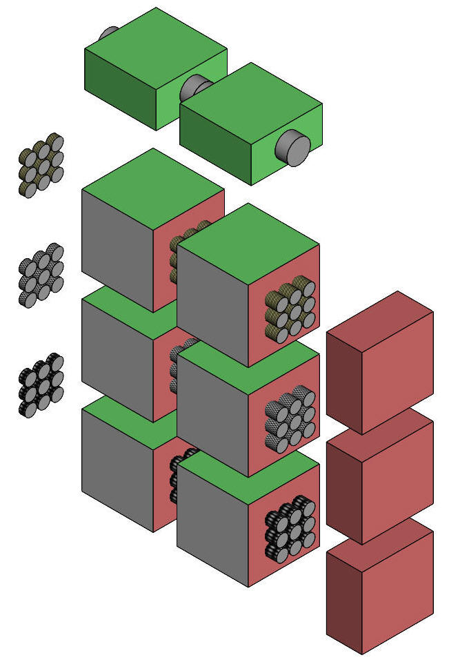
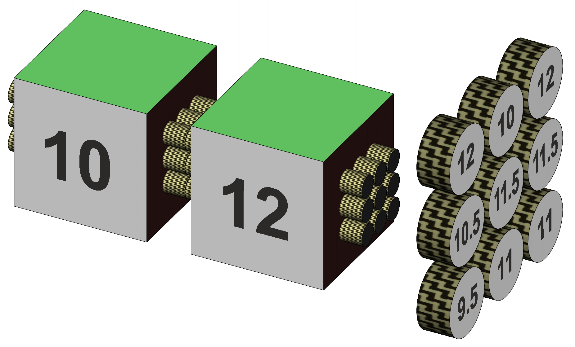
Previous page dealt with Two way factorial anova. Two-way anova, repeated measures on one factorA group of 9 subjects each drink a preparation containing amino acids, proteins, and peptides. The drink tastes (and smells) medicinal. A second group of 9 subjects drink a preparation that tastes medicinal but contains no active ingredients. A third group of 9 subjects drink tea. All 27 subjects undertake a memory test before their drink, and then again a short interval after their drink. Notice the repeated measures – the same subjects are tested before and after their drink. This is said to be repeated measures on one factor (§1). Figure 1 illustrates the design of the data, showing the array of subject average scores on the left..
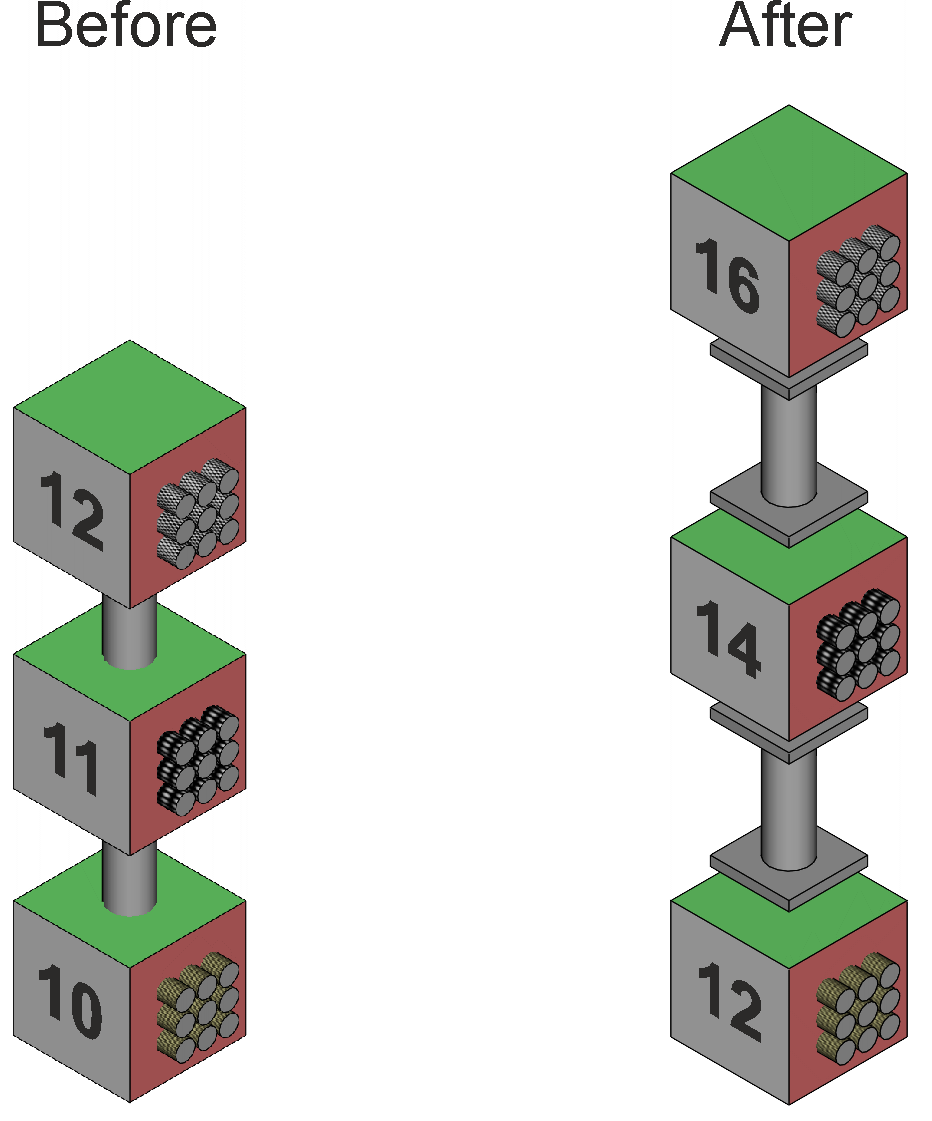
Figure 1. Representation of a two-way anova with
repeated measures on one (the green) factor. The repeated measures are indicated by the tubes or cylinders. A set of nine tubes are shown for a group of 9 subjects. The tubes in one set are patterned similarly, and differently in other sets (might be difficult to see here in Figure 1, perhaps more easily in Figure 4 below). The same subjects and the same pattern is shown in the before and after cubes for a particular drink. Each drink has a different group of subjects with a different pattern. The green Before and After means are connected by a single larger cylinder that is un-patterned. This is because their means are calculated over three different subjects, so while individual subjects cannot be identified, they are based on the same 3 groups of subjects. The green Pre-post factor is a within-subjects factor. The red Tea, Protein, and Inactive means are not connected because each is based upon a different group of subjects, and hence the Drink factor is a between-subjects factor. The test scores are shown in Table 1. Notice also that the data is the same as that for the two-way independent samples anova that has been re-arranged as three groups of subjects. Table 1. Memory test scores for 27 subjects, before and after 3 drink types.
The question here is whether the protein drink improves the memory of the subjects compared to an inactive drink or to tea. The subjects provide their own control data, in that their baseline memory is tested before their drink, so that their test afterwards gives a better picture of whether the drink has any effect. This is a classic pre- and post-test experiment, and works well provided that the subjects do not learn or remember anything from the pre-test that modifies their post-test scores. It also works well as an experimental design, but only on the assumption that the subjects show consistency in their memory scores from Before to After, that is, their Before and After scores are "adequately" correlated. The labels for the factors are "Drink" and "Pre-post", and their levels are "Tea", "Protein", and "Inactive", and "Before" and "After". The measure is "Memory". The question could be answered by calculating a change score for each subject, being their After score minus their Before score, and then asking whether the change shown by the protein drink is larger than that shown by the tea or inactive drinks. As discussed in the page on Two dependent samples, this is a natural and straightforward approach to analysing any pre-post or before-after data, but it has a hidden and therefore problematic issue — relating any data to the change score can give spurious results. In addition, analysing the change scores does not allow an answer to the preliminary question of whether the subjects in each group started off with equal or similar memory scores. If the average pre-test score of each group is different, then any apparent increase (or decrease) in the average post-test score of a group could be due to its higher (or lower) pre-test rather than due to the effect of the group's drink. These two problems with analysing change scores are addressed by not using a one-way analysis on change scores but instead investigating the interaction effect using a two-way analysis. We remember that a significant interaction suggests the effects of one factor depend upon the levels of the second factor. In the case of our data, significant interaction suggests the differences between Before and After scores depend upon whether the subjects took Tea, Protein, or Inactive drinks. This gives the answer to the question whether the protein drink improves the memory of our subjects compared to an inactive drink or to tea, and importantly this answer does not depend on any differences between the groups' baseline memory scores before the experiment. The follow-on analyses of main effects (insignificant interaction) or simple main effects (significant interaction) and related pairwise comparisons identify the sources of any differences in more detail, and in particular identify whether the group baselines were similar or significantly different. §1 The "two way with repeated measures on one factor" design is one of a range of designs depending on the factors which have repeated measures, if any. The other designs are "two way with no repeated measures" and "two way with repeated measures on both factors". We call the two-way with no repeated measures a "two way factorial", while some authors use "two way completely randomised". Some authors call a "two way with repeated measures on both factors" a "randomised blocks" design, and this suggests a common name of "mixed" for "two way with repeated measures on one factor". Authors with an agricultural background call "two way with repeated measures on one factor" a "split plot factorial" design.
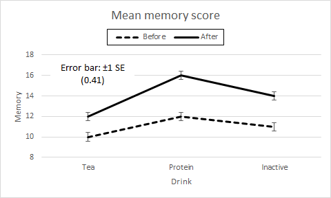
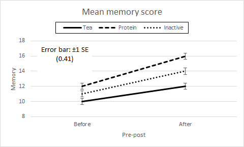
Profile plotsWe know to always plot our data. From the cell means we draw Pre-post × Drink and Drink × Pre-post profile plots which are the same as for the Two way factorial anova data.
Figure 2. Profile plots of Drink × Pre-post and Pre-post × Drink.
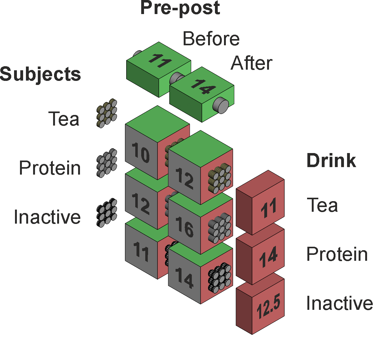
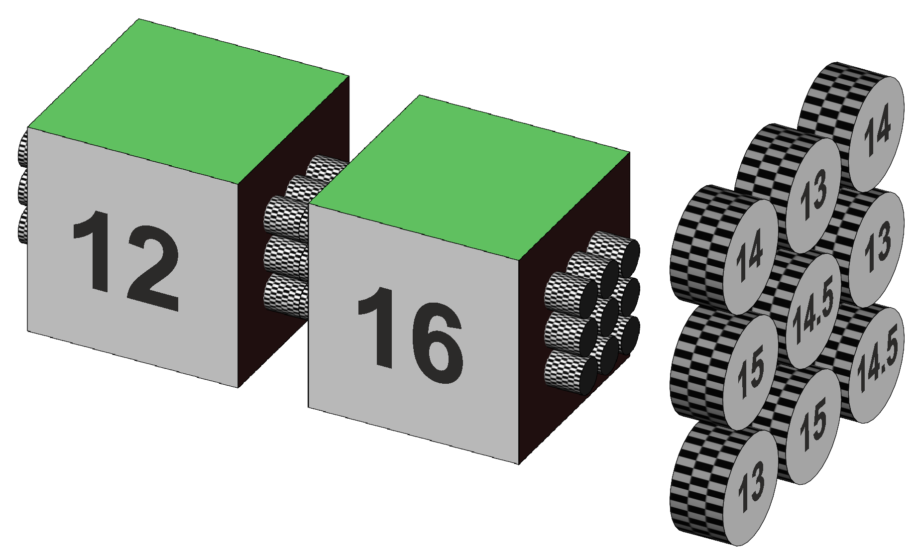
Effect means and variancesThe cell, Drink, and Pre-post means are the same as for the Two way factorial anova data. We provide the tables of means in a slightly different arrangement here and give them slightly different labels, as shown in Table 2 and illustrated in Figure 3.
Figure 3. Illustration of the cell and factor means. Table 2. Memory test mean scores for Drink, Pre-post, and Drink × Pre-post.
The following are the general principles of calculating SS, MS, and df for an effect using means.
We calculated MS, SS, and df in detail for our effects in the Two way factorial anova page, and summarise the calculations here. The means of the Drink, Pre-Post, and Drink×Pre-Post data are labelled [D], [P], and [DP]. Their sums of squares, calculated according to steps 1a to 1c, are labelled SS[D], SS[P], and SS[DP] and are 81.0, 121.5, and 211.5, while their df are labelled df[D], df[P], and df[DP] and are 2, 1, and 5. According to step 1d, the calculations for the main effects are complete, so SS(Drink) = SS[D] = 81.0 with df(Drink) = df[D] = 2, hence MS(Drink) = 40.5; and SS(Pre-Post) = SS[P] = 121.5 with df(Pre-Post) = df[P] = 1, hence MS(Pre-Post) = 121.5. According to step 1d, the calculation for the interaction effect requires steps 2a to 2c, where SS(Drink×Pre-Post) = SS[DP] – SS(Drink) – SS(Pre-post) = 211.5 – 81.0 – 121.5 = 9, df(Drink×Pre-Post) = df[DP] – df(Drink) – df(Pre-post) = 5 – 2 – 1 = 2, and so MS(Drink×Pre-Post) = SS(Drink×Pre-Post) / df(Drink×Pre-Post) = 9 / 2 = 4.5. It is useful to identify the pattern here. We notice that square brackets, [], are used to denote means of the data, and round brackets, (), are used to denote the effects we test for significance. From the effect means labelled [D], [P], and [DP] we calculate their sums of squares which we can label SS[D], SS[P], and SS[DP]. We see that SS(Drink×Pre-post) = SS[DP] – SS(Drink) – SS(Pre-post). We can generalise our ability to partition the sums of squares for any interaction effect, say Z×W, by noting that we subtract SS(Z) and SS(W) from SS[ZW] to yield SS(Z×W).
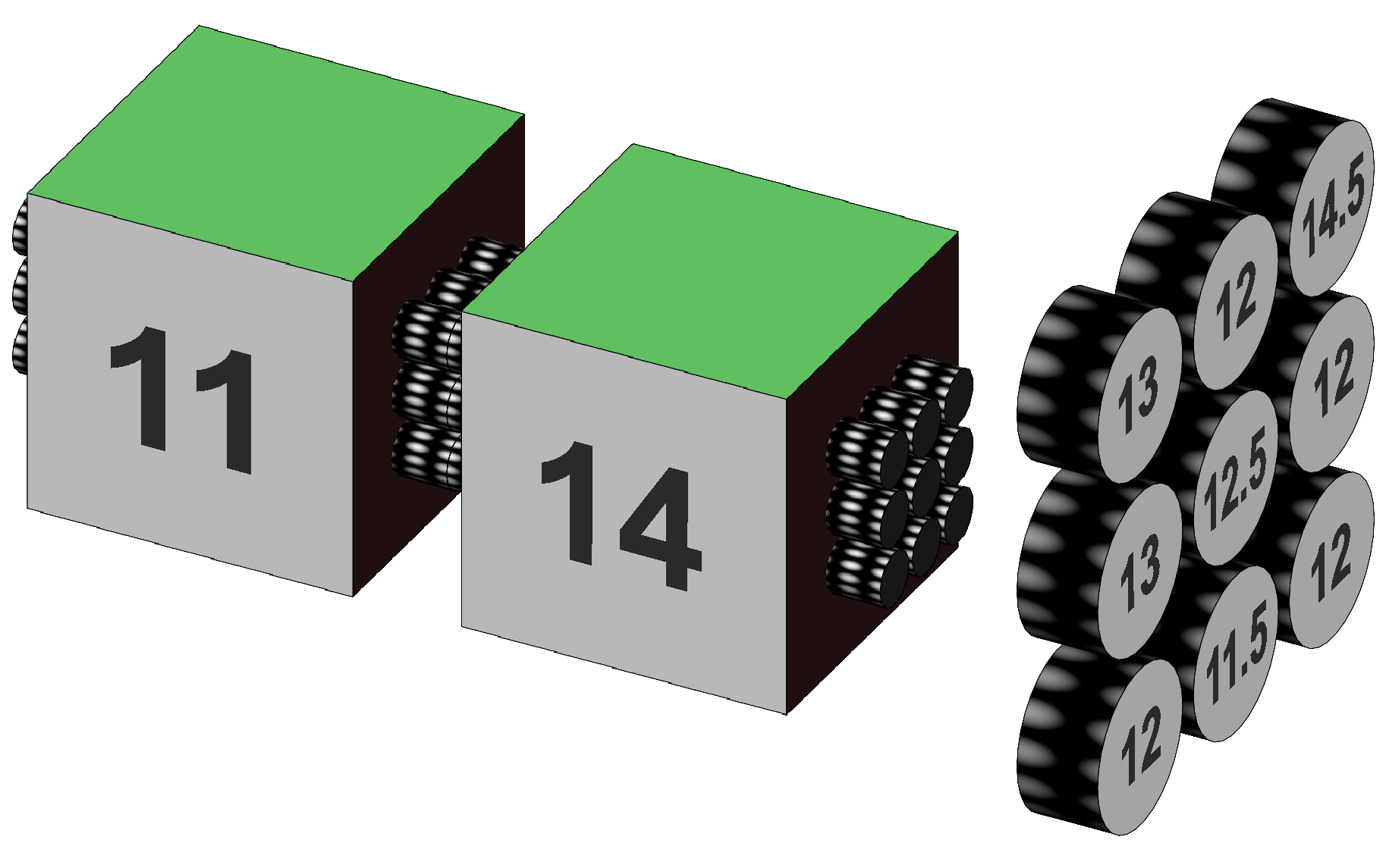
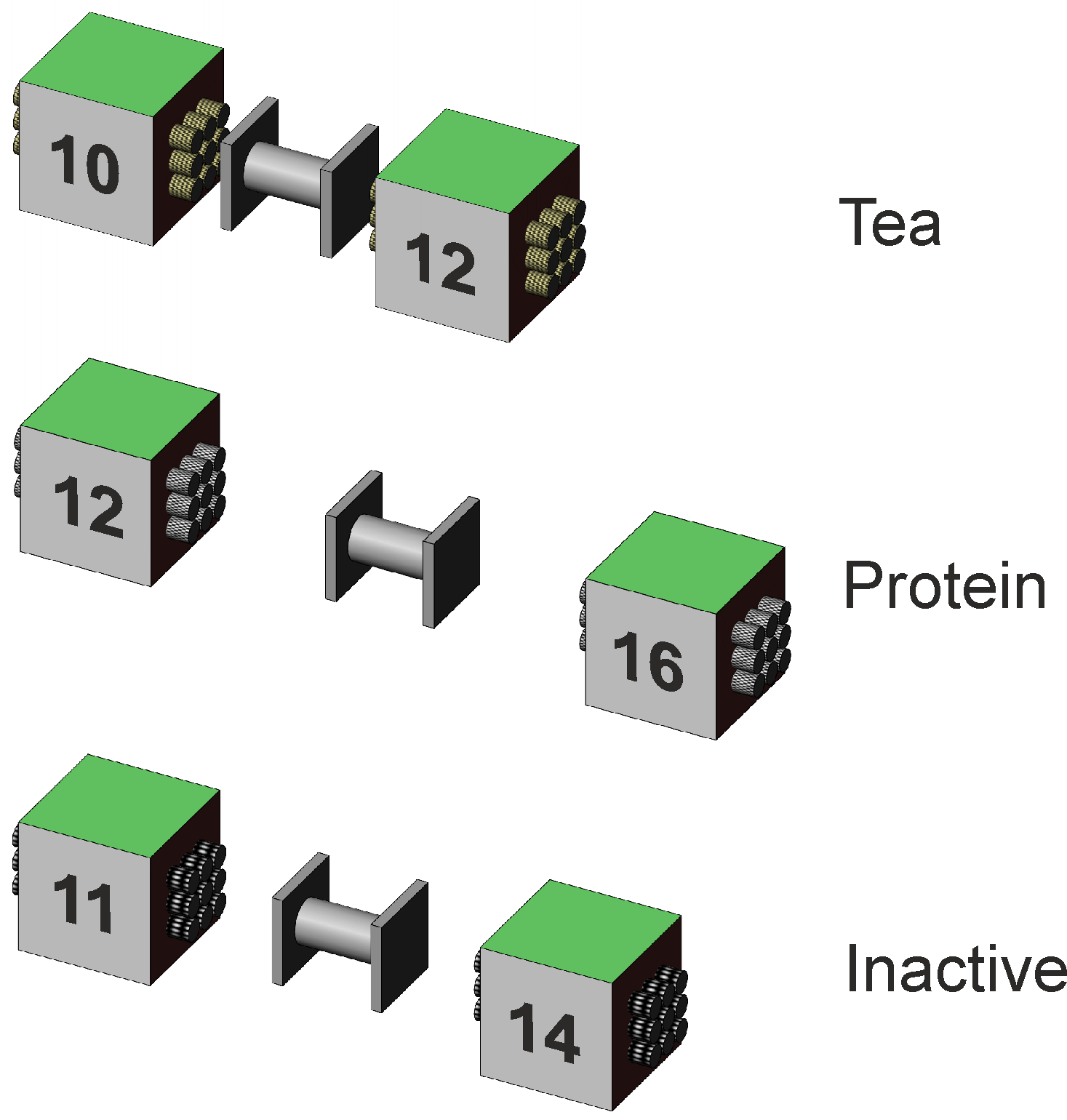
Error variancesWe begin with the calculation of error variation, as detailed in the One way anova (independent samples section) and Two way factorial anova pages by taking the average variance of the data in each cell, which for our data is (1.5 + 1.5 + 1.5 + 1.5 + 1.5 + 1.5) / 6 = 1.5. The df is the sum of the df for each cell, which for our data is 6 · (n–1) = 4 · 8 = 48. Error variation, expressed as SS, is 48 · 1.5 = 72. For our data, however, the subjects provide their baseline memory before their drink, so that their test afterwards gives a better picture of whether the drink has any effect. The dependent samples section in the One way anova page shows how to account for the portion of the sample variation that can be attributed to variation between our subjects, and how to deduct it from the cells' variation to give the remaining, smaller, variation is that shown within our subjects. We remember that the between-subjects SS is calculated from the variation shown by the subjects' average scores across Before and After, and is deducted from the cells' error SS to give the within subjects variation that can also be called residual. Table 3 shows the average subjects' scores across Before and After for each of the groups, the calculated variance of the average for each group, and the calculated SS given that each average is based upon two scores and the df for a group of subjects is 9 – 1 = 6. The subject average scores are illustrated in Figure 4.
Figure 4. Depiction of subject average scores for each group of subjects associated with Tea, Protein, and Inactive. Table 3. Memory test mean scores for subjects.
The total SS for subjects is 12 + 11 + 13 = 36, and df is 8 + 8 + 8 = 24. These are deducted from SS(Cells) and df(Cells) to yield SS(Resid) = 72 - 36 = 36 with df(Resid) = 48 - 24 = 24, hence MS(Resid) = 36/24 = 1.5. We change our terminology to refer to the variation we have labelled as "subjects" to be, more accurately, the variation "between subjects", hence SS(Between subjects) = 36, df(Between subjects) = 24, and MS(Between subjects) = 1.5 (§2). There are a number of names for these error terms, depending on the domain of application and on the statistical school being followed. The SS after deduction of SS(Between subjects) from SS(Cells) can be called SS(Residual), SS(Within), SS(Within subjects), SS(Error within), SS(B×subjects), or SS(B×SwG). SS(Between subjects) can be called SS(Subjects), SS(Error(Subjects)), SS(Error between), SS(Subjects within groups), or SS(SwG). We remember that a repeated measures experimental design is only efficient if the subjects show "appreciable" consistency from one measurement to another. If there is little or no consistency, there is little or no difference between MS(within subjects) and MS(between subjects) and both are more or less equal to MS(Cells). Hence there is no benefit to partitioning the error variation into between and within subjects, while the costs remain — the tests of the main and interaction effects suffer from smaller df, higher critical values, and lower power. Where there is little or no consistency between the subject scores, the data may be better analysed as a two-way factorial, ignoring the repeated measures. Remember to explain this tactic for an alert reviewer. §2 The MS of the two error terms are equal to each other and are equal to MS(Cells), 1.5. This is because the subjects show zero correlation overall between their Before and After scores. The coefficient of correlation between the Before and After scores is r = 0.0 for the Tea group, r = -0.08 for the Protein group, and r = 0.08 for the Inactive group, so effectively zero when taken overall. When there is some correlation between Before and After, the two error terms have different values.
Anova summary for repeated measures on one factorWe have three effects to test in a two factor anova — the main effects of each factor, MS(A) and MS(B), and their interaction effect, MS(A×B). We have two measures of error, MS(Between subjects) and MS(Within subjects), and the issue is the appropriate error term for each test. The repeated measures are across the Pre-post factor from Before to After, that is, differences between Before and After are within subjects. This suggests that MS(Pre-post) is appropriately tested by MS(Within subjects), that is, MS(Residual) for our data. There are no repeated measures across the Drink factor, that is, differences between Tea, Protein, and Inactive drinks are between the subject groups. This suggests that MS(Drink) is appropriately tested by MS(Between subjects). The interaction effect is considered a within-subjects effect, and hence is tested by the within-subjects error term. MS(Drink×Pre-post) is tested by MS(Within subjects), that is, MS(Residual) (§3). The results of the analysis are shown in Table 4. Note the table is laid out, by convention, with the between-subjects results first and labelled "Between subjects", followed by the within-subjects results labelled "Within subjects". This convention usually permits the correct identification of which error term is which no matter if they have labels not previously seen or are placed elsewhere in the table. Note that SPSS presents its repeated measures output the other way around, within-subjects before between-subjects. Table 4. Anova summary table for repeated measures on one factor.
These numerical results are almost exactly the same as the results seen in the Two way factorial anova page, as note §1 explains. Their interpretation is also the same, which we can summarise using the names and labels for the factors and levels of the present data. We always start with the interpretation of the interaction effect. Here we see that, with α = .05, it is not significant, p = .069. This tells us that the drinks have similar effect trends, that is, not significantly different, from Before to After, and that the differences in the Pre-post measures are similar, that is, not significantly different, for Tea, Protein, and Inactive drinks. The main effects can now be interpreted. The significant Drink effects tells us that there are significant differences between the drinks overall, and pairwise comparisons are needed to identify where these differences lie. At the least, the largest drink mean is significantly larger than the smallest drink mean. The significant Pre-post effect tells us that there is a significant difference between the Before and After mean scores overall. There is no need for a pairwise comparison, it merely remains to inspect the profile plot or the table of Pre-post means to see which of the means is the one that is significantly higher, and it is the After mean in our data. The main effect profile plots have the same profiles as those shown in the Two way factorial anova, so are not reproduced here, but the error bars are different (§4). We note that the SE of the main effect means shown on the within-subjects means plot should be given by the square root of MS(Within subjects) / qn, where q is the number of levels of the within-subjects factor. For our data, the within-subjects factor is Pre-post with two levels, Before and After, hence SE = √ (1.5 / 27) = 0.24 for each of the Before and After means plotted. In contrast, the SE of the main effect means shown on the between-subjects mean plot should be given by the square root of MS(Between subjects) / pn, where p is the number of levels of the between-subjects factor. For our data, the between-subjects factor is Drink with three levels, Tea, Protein, and Inactive, hence SE = √ (1.5 / 18) = 0.29 for these means. By coincidence, as explained in the first part of Note §1, the MS value is 1.5 for both of the error bars, but in general they will have different values. We remember that a main effect is overall the levels of the other factor, so the interpretation of the significant Pre-post main effect is that the After means of all the drinks are significantly higher than their Before means by similar amounts. The main effect of Drink is more awkward to interpret because of the structure of the experiment. The significant Drink effect is that the Tea, Protein, and Inactive means taken on average across the Before and After scores are different by similar amounts. Taking an average score of a drink across Before and After is not particularly meaningful in the context of this experiment, and there is little value in analysing the significant Drink main effect further. This is because of the lack of interaction between Drink and Pre-post, and this lack strongly illustrates the way in which the interaction effect of a two way anova tells us exactly what we need to know about the effects of Drink on the change in scores from the baseline Before drinks memory test to the After drinks memory test. Nevertheless, we examine pairwise comparisons for both Drink and Pre-post in the next section because their error terms are different in the case of repeated measures, and it is important to know the construction of the desired LSD t-tests when they are meaningful. If the data is the outcome of an actual experiment, an investigator is always interested in a "suggestive" result. We know that α = .05 is a conventional level of significance, and an investigator is free to employ a different value, for example α = .10, to see where it might lead. This would be for their own interest and to inform their planning of future experiments, since no reputable journal publishes results which are not significant at the conventional level of α = .05 or, particularly in medicine, at α = .01. The interaction effect is "suggestive" on this account. §3 The exact justification for using MS(Within subjects) to test the interaction effect which, on the face of it, is only partially within subjects, is given by a mathematical derivation outside the scope of our conceptual explanation. §4 Note that the error bar SEs of the various cell means shown on the interaction profile plots is given by s / √n for each cell if their standard deviations are markedly different, or by using the square root of MS(Cells) / n for each, where MS(Cells) is the average of the cell variances. For our data, we use SE = √ (1.5 / 9) = 0.41 for each cell mean. This is different from the provision of the error bars on the main effects profile plots, where the SE depends on whether the effects are within subjects or between subjects.
Pairwise comparisons for main effects in repeated measures on one factorWe consider here the follow-on to a significant main effect, given an insignificant interaction. (We remember that if the interaction is significant, the main effects are ignored, and any pairwise comparisons are what we might call "simple" because they are follow-ups to significant simple main effects.) The follow-up to a significant between-subjects main effect is similar to a within-subjects main effect, in that we examine the differences between a pair of main effect means using a t-test, but it is different in that the standard error for the t-test is different. Differences between within-subjects main effect means are tested using MS(Within subjects), that is, MS(Residual) for our data. Differences shown by between-subjects main effect means are tested using MS(Between subjects). The degrees of freedom for these tests are df(Residual) or df(Between subjects) as appropriate. The Drink main effect is significant. Because the Drink effect is between subjects, the t-tests for the differences between the Tea, Protein, and Inactive drinks use MS(Between subjects). From Table 2, the main effect means are 11, 14, and 12.5. At the least, we know that the mean memory score for Tea overall is significantly lower than that for Protein, so we can test another pair, such as the difference between Tea and Inactive overall. The difference is 11 – 12.5 = –1.5. The standard error for a difference between independent means each based on n items of data is given by √ (2MS / n) where MS here is MS(Between subjects) = 1.5, hence SEdiff = √ (2 · 1.5 / 18) = 0.41. For this test, t = –1.5 / 0.41 = –3.67 with df = df(Between subjects) = 24, and we find p = .001.
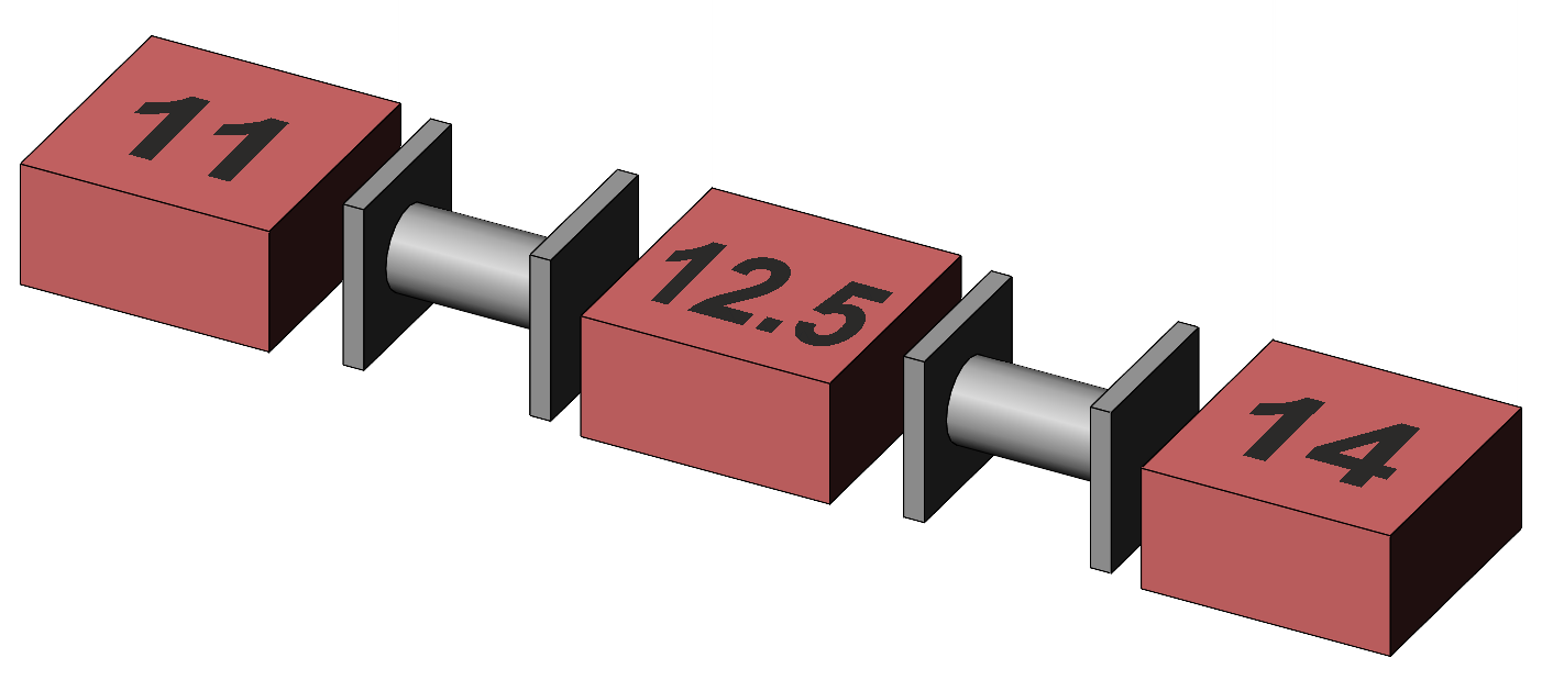
Figure 5. Representation of the pairwise comparisons between Factor A, Drink, main effect means with differences relative to 2·SEdiff. The Pre-post main effect is significant. Because the Pre-post effect is within subjects, the t-test for the difference between the Before and After means overall uses MS(Resid). From Table 2, the main effect means are 11 and 14. Of course, there is in fact no need to conduct a pairwise comparison because the Pre-post factor comprises only two levels and their difference is tested by the main effect F ratio directly. It is interesting to conduct the t-test anyway — the difference is 10 – 14 = –3, the standard error of the difference is given by √ (2MS / n) = √ (2 · MS(Residual) / 27) = 0.33, hence t = –3 / 0.33 = –9 with df = df(Residual) = 24, and we find p <.001. We remember that t2(df) = F(1,df) and see that –92 = 81 = F from Table 4 as expected. The pairwise comparison for Before and After is illustrated in Figure 6. Note the cylinders in the Factor B means, reminding us that their difference is within subjects and that the SEdiff is therefore based on MS(within subjects).
Figure 6. Representation of the pairwise comparison between Factor B, Pre-post, main effect means with differences relative to 2·SEdiff.
Appreciable within-subjects correlationThe data we have analysed above is artificial in order to bring out points of interest. For the following analysis, again to bring out points of interest, the set of data has been re-arranged so that there is appreciable correlation between the Before and After scores of the subjects, as per Table 5. Table 5. Memory test mean scores for subjects ("appreciable" correlation between Pre-post scores).
The coefficient of correlation between the Before and After scores is r = 0.5 for the Tea group, r = 0.58 for the Protein group, and r = 0.42 for the Inactive group, so 0.50 when taken overall. There is no change to the cell means, factor means, or cell variances. The consistency of the subjects' scores from Before to After only affects the error terms, such that SS(Between subjects) is 18 + 19 + 17 = 54 and MS(Between subjects) = 2.25, while SS(Residual) is 18 and MS(Residual) = 0.75, with corresponding changes to the effect F ratios. Table 6. Anova summary table for repeated measures on one factor ("appreciable" correlation between Pre-post scores).
We see that the interaction is declared significant, and we therefore proceed with the analysis of simple main effects. The overall concepts for simple main effects are as for any factorial analysis of variance, but the change is in the detail of how the error terms are used for repeated measures data.
Simple main effects in repeated measures on one factorThere are two sets of simple main effects, one for each factor which corresponds to one of the interaction profile plots. Both sets of simple main effects are constructed following a significant interaction effect. One set examines the simple main effects of Pre-post for each of the three drinks separately, and one set examines the simple main effects of Drink for each of the Pre-post levels of Before and After separately. The simple main effects of Pre-post for Tea are given by a one-way anova of the Before and After means for Tea, being 10 and 12; for the Protein means 12 and 16; and for the Inactive means of 11 and 14. The issue in repeated measures designs is the selection of the correct error term, and this requires particular attention in the analysis of simple main effects. We remember from the analysis of simple main effects in the Two way factorial anova that each simple main effect is a combination of the main effect and the interaction effect. The combination is that the sums of squares add up, and this is illustrated in Table 7 for two factors Z and W with 2 and 3 levels respectively. Table 7. Composition of simple main effect sums of squares.
We consider the situation where Z is a between-subjects factor and W is a within-subjects factor, and lay out the error terms used to test the main and interaction effects, as in Table 8. Table 8. Error terms for effects in the anova with repeated measures on one factor
The key observation is to see that the simple main effects of W are a combination of the W and Z×W effects, both of which are tested by the same error term, MS(Residual). By contrast, the simple main effects of Z are a combination of the Z and Z×W effects, where Z is tested by MS(Between subjects) and Z×W is tested by a different term, MS(Residual). We conclude that, in order to test the simple main effects of Z, we require an error term which is the combination of MS(Between subjects) and MS(Residual). This is a general approach to testing any simple effect and the required error term is often said to be Pooled, denoted as MS(Pooled). It is very simply made up, SS(Pooled) = SS(Between subjects) + SS(Residual) and df(Pooled) = df(Between subjects) + df(Residual), yielding MS(Pooled) = SS(Pooled) / df(Pooled). For our data, SS(Pooled) = 54 + 18 = 72, df(Pooled) = 24 + 24 = 48, and hence MS(Pooled) = 72 / 48 = 1.5 (§5). For the simple main effects of Pre-post, we note that the Pre-post main effect, MS(Pre-post), is a within-subjects effect, the interaction effect, MS(Drink×Pre-post), is also a within-subjects effect, and hence the required error term is MS(Residual) from the two-way anova. The F ratio degrees of freedom are 1 and 24, being the df for the simple effect (two means, df = 2 – 1 = 1) and the df for MS(Residual) of 24. We remember that the MS of an effect is given by multiplying the variance of its means by the number of data items which make up each mean, here 9. The summary table of the simple main effects for Pre-post is shown in Table 8. Table 9. Simple main effects for Pre-post.
All three simple main effects of Pre-post are significant, suggesting that the Tea, Protein, and Inactive drinks each show a difference from Before to After. Because there are only two levels of the Pre-post factor, the actual nature of the difference is immediately given by inspecting the interaction profile plots or the table of cell means, where we see that, for each drink, the After mean is significantly higher than the Before mean. Each drink seems to result in a significant increase in the memory test scores of our subjects. If this factor comprised three or more levels, the follow-on is to conduct "simple" pairwise comparisons for each simple main effect. Later in this section we identify the correct standard error in the t-tests for such "simple" pairwise comparisons using the insights of Table 7 and Table 8. As a check, adding up the SS for the Pre-post simple main effects gives 18 + 72 + 40.5 = 130.5, which is the value given by adding up SS(Pre-post) and SS(Interaction) = 121.5 + 9 = 130.5. The simple main effects of Drink for each level of Pre-post are given by a one-way anova of the Before means of Tea, Protein, and Inactive, being 10, 12, and 11, and a second one-way anova of the After means, 12, 16, and 14. Drink is a between-subjects effect, but the interaction of Drink with Pre-post is a within-subjects effect, and so the appropriate error term is MS(Pooled). For our data, MS(Pooled) = 1.5 with df(Pooled) = 48. The F ratio degrees of freedom are 2 and 48, being the df for the simple effect (three means, df = 3 – 1 = 2) and the df for MS(Pooled), 48. We remember that the MS of an effect is given by multiplying the variance of its means by the number of data items which make up each mean, here 9. The summary table of the simple main effects for Drink is shown in Table 10. Table 10. Simple main effects for Drink.
The two simple main effects of Drink are significant, suggesting that the Tea, Protein, and Inactive drinks show a significant difference in their Before means, p = .005, and also show a significant difference in their After means, p <.001. The first result is unwelcome, because it suggests that the drink groups have different baseline (Before) memory scores. At the least, we can say that the highest Before mean is significantly different from the lowest Before mean — that the Tea Before mean of 10 is significantly lower than the Protein Before mean of 12. We need pairwise comparisons to tells us whether the Tea Before mean is different from the Inactive Before mean, and whether the Protein Before mean is different from the Inactive Before mean. The second result is probably the one we hope for as the investigator, telling us that the After means are significantly different. At the least we can say that the highest After mean is significantly different from the lowest After mean — that the Tea After mean of 12 is significantly lower than the Protein After mean of 16 — and that pairwise comparisons are needed to tell us about the other After mean differences. Adding up the variation, that is the SS, for the Drink simple main effects gives 18 + 72 = 90, and similarly the total df is 2 + 2 = 4. We can see that these are the values given by adding up SS(Drink) and SS(Interaction) = 81 + 9 = 90 and df(Drink) and df(Interaction) = 2 + 2 = 4. §5 We remember that SS(Cells) was 72, and that it was partitioned into between-subjects and within-subjects components. Combining SS(Between subjects) and SS(Resid) in our example simply takes us back to SS(Cells) and thus MS(Pooled) = MS(Cells).
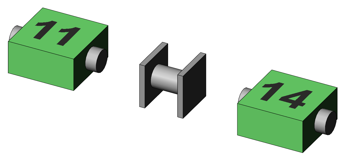
"Simple" pairwise comparisons following significant simple main effectsThe issue in pairwise comparisons for repeated measures data is the correct choice of the standard error in the t-tests. We refer to the choices made in the analysis of the simple main effects, and continue with those choices for "simple" pairwise comparisons. From Table 10, the simple main effects anova shows a significant simple main effect for the Drink factor at Pre-post = Before. We compare the mean Protein Before memory score with the mean Inactive Before and Tea Before means, and the mean Inactive Before with Tea Before. We remember that conducting separate significance tests, 3 for each family in this case, inflates the family-wise Type I error rate; that simple LSD t-tests are acceptable given no more that 3 means being compared; and that Sidak or Tukey tests or corrections are otherwise indicated. A t-test for the difference between two cell means uses SEdiff calculated as √ (2 · MS / 9), where the value of MS is given by that used in the test of the parent simple main effect and the value of "9" is the cell n. Table 10 shows that MS(Pooled) is used to test the Drink simple main effects, and hence the pairwise comparisons use MS(Pooled) as the basis of the SEdiff to test difference between drinks at each level of Pre-post, that is, Before and After. MS(Pooled) = 1.5 hence SEdiff = √ (2 · 1.5 / 9) = 0.58. The df for the t-test are as for MS(Pooled), 48. For the difference between Tea and Inactive when Pre-post is Before we have t = (10 – 11) / 0.58 = –1.73, p = .09; between Inactive and Protein we have t = (11 – 12) / 0.58 = –1.73, p = .09; and between Tea and Protein we have t = (10 – 12) / 0.58 = –3.46, p = .001. We see that, for the Before means, only the difference between Tea and Protein is significant. The differences between Tea and Inactive, and Inactive and Protein, are not significant. A check with the Drink × Pre-post profile plot shows the relatively small gaps between the Before Drink means, consistent with the pairwise comparisons. Following the significant simple main effect for the Drink factor at Pre-post = After, we compare the mean Protein After memory score with the mean Inactive After and Tea After scores, and the mean Inactive After with Tea After. For the comparison between Tea and Inactive when Pre-post is After we have t = (12 – 14) / 0.58 = –3.46, p < .001; between Inactive and Protein we have t = (14 – 16) / 0.58 = –3.46, p < .001; and between Tea and Protein we have t = (12 – 16) / 0.58 = –6.92, p < .001. We see that, for the After means, all the differences between Drink are significant. A check with the Drink × Pre-post profile plot shows the relatively large gaps between the After Drink means, consistent with the pairwise comparisons. Figure 7 illustrates the "simple" pairwise comparisons between the Drink means at Pre-post = Before, and between the Drink means at Pre-post = After. The cells have been ordered according to their means. Note that the comparisons are between subjects, that is, the subject tubes do not connect from one cell mean to another. This signifies that SEdiff for these comparisons is based upon MS(Pooled).
Figure 7. Depiction of pairwise comparisons between
Drink at each level of Pre-post, differences relative to 2·SEdiff.
From Table 9, the simple main effects anovas for the Pre-post factor show a significant simple main effect for each of Pre-post for Tea, Protein, and Inactive drinks. We can compare the mean Tea Before memory score with the mean Tea After, and so on for the Protein and Inactive drinks. We calculate a pairwise comparison for the Tea means in order to illustrate the general principles. We note that these pairwise comparisons are not necessary; if there is a significant simple main effect for a factor with two levels it is immediately clear from the profile plot or the cell means which mean is significantly higher than which other. We see that MS(Residual) is used to test the Pre-post simple main effects, and hence the Pre-post pairwise comparisons use MS(Residual). MS(Residual) = 0.75 hence SEdiff = √ (2 · 0.75 / 9) = 0.41. We note the division by 9 because each cell mean is based upon 9 scores. The df for the t-test are as for MS(Residual), 24. For the comparison between Tea Before and Tea After we have t = (10 – 12) / 0.41 = –4.90, p <.001. We remember that t2(df) = F(1,df) and see that –4.92 = 24 = F from Table 8 as expected. Figure 8 illustrates the "simple" pairwise comparisons between Before and After at each level of Drink. Note the alignment of the subject tubes connecting Before to After, signifying that the comparisons are within subjects and hence that SEdiff is based on MS(Residual).
Figure 8. Depiction of pairwise comparisons
between Pre-post at each level of Drink, differences relative to 2·SEdiff.
From the repeated measures section of the One way anova page we may remember the availability of specific pairwise comparisons which use the correlation between the pairs of factor levels involved. The technique is available for the two-way repeated measures design for pairwise and "simple" pairwise comparisons between main effect or simple main effect means of a within-subjects factor with more than 2 levels. We do not rehearse their application here, but mention them because some statistical analysis software packages, such as SPSS, apply these specific tests, and their results may not agree with the results expected for a more general test which uses the average correlation, equivalent to using unadjusted MS(Residual).
SummaryThe analysis of the two-way anova with repeated measures on one factor follows the same procedures as the two-way factorial anova in the calculation of main and interaction SS, df, and MS. The difference is that the repeated measures design allows the separation of within and between subjects' error variation. The issue in the repeated measures anova is the choice of the correct error MS for the main and interaction effects and for the simple main effects, and the choice of the correct SE in the pairwise comparisons t-tests following significant main effects or significant simple main effects. The between-subjects error variation may be called SS(Subjects) and the within-subjects error variation may be called SS(Residual) to remind us how they are calculated. SS(Subj) is the variation seen in the mean scores of the subjects and is subtracted from the variation seen in the cells, SS(Cells), to give SS(Resid). Similarly, the degrees of freedom for the subjects, df(Subj), is subtracted from df(Cells) to give df(Resid). Hence MS(Subj) = SS(Subj)/df(Subj) and MS(Resid) = SS(Resid)/df(Resid). Other authors call between-subjects and within-subjects error variation by other terms when they are calculated by other, more mathematically efficient, ways or when they occur in different domains. Considering two factors Z and W where repeated measures are taken from the same subjects at each level of W, Z is a between-subjects factor and W is a within-subjects factor. The factor main effects MS(Z) and MS(W) are tested by their appropriate error term, MS(Subj) for between-subjects MS(Z), and MS(Resid) for within-subjects MS(W). The interaction effect MS(Z×W) is considered a within-subjects effect and so is tested by MS(Resid). Given an insignificant interaction, significant main effects may be analysed further using pairwise comparisons. The appropriate SEdiff for the t-tests of differences between factor Z main effect means is based on MS(Subj) since Z is between subjects, and the appropriate SEdiff for the t-tests of differences between factor W main effect means is based on MS(Resid) since W is within subjects. Given a significant interaction, analysis turns to the simple main effects of Z at each level of W, being MS(Z at W1), MS(Z at W2), and so on, and to the simple main effects of W at each level of Z, MS(W at Z1), MS(W at Z2), and so on. The variation analysed by the simple main effects of a factor comprises the variation of that factor's main effect plus the interaction variation, such that SS(Z) + SS(Z×W) = MS(Z at W1) + MS(Z at W2) + ... + MS(Z at Wq) and similarly SS(W) + SS(Z×W) = MS(W at Z1) + MS(W at Z2) + ... + MS(W at Zp). In the case of the simple main effects of W, the variation shown by SS(W) and SS(Z×W) are both within subjects, and the appropriate error term for any MS(W at Zi) is MS(Resid). However, in the case of the simple main effects of Z, the variation shown by SS(Z) and SS(Z×W) is between subjects for Z and uses MS(Subj) but within subjects for Z×W which uses MS(Resid). Testing the simple main effects of Z requires an error term which combines SS(Subj) and SS(Resid); the combination is called "Pooled" and is given as SS(Pooled) = SS(Subj) + SS(Resid), correspondingly df(Pooled) = df(Subj) + df(Resid), and so the required error term MS(Pooled) = SS(Pooled)/df(Pooled). The appropriate error term for any MS(Z at Wj) is MS(Pooled). A significant simple main effect may be analysed further using pairwise comparisons. The appropriate SEdiff for the t-tests for differences between factor Z simple main effect means is based on MS(Pooled) because the Z simple main effect is tested using MS(Pooled). The appropriate SEdiff for the t-tests for differences between factor W simple main effect means is based on MS(Resid) because the W simple main effect is tested using MS(Resid). Next page deals with Two way rep meas both factors.
| |||||||||||||||||||||||||||||||||||||||||||||||||||||||||||||||||||||||||||||||||||||||||||||||||||||||||||||||||||||||||||||||||||||||||||||||||||||||||||||||||||||||||||||||||||||||||||||||||||||||||||||||||||||||||||||||||||||||||||||||||||||||||||||||||||||||||||||||||||||||||||||||||||||||||||||||||||||||||||||||||||||||||||||||||||||||||||||||||||||||||||||||||||||||||||||||||||||||||||||||||||||||||||||||||||||||||||||||||||||||||||||||||||||||||||||||||||||||||||||||||||||||||||||||||||||||||||||||||||||||||||||||||||||||||||||||||||||||||||||||||||||||||
|
©2025 Lester Gilbert |