![]()
![]()
![]()
![]()
![]()
![]()
![]()
|
|
|
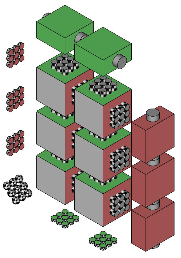
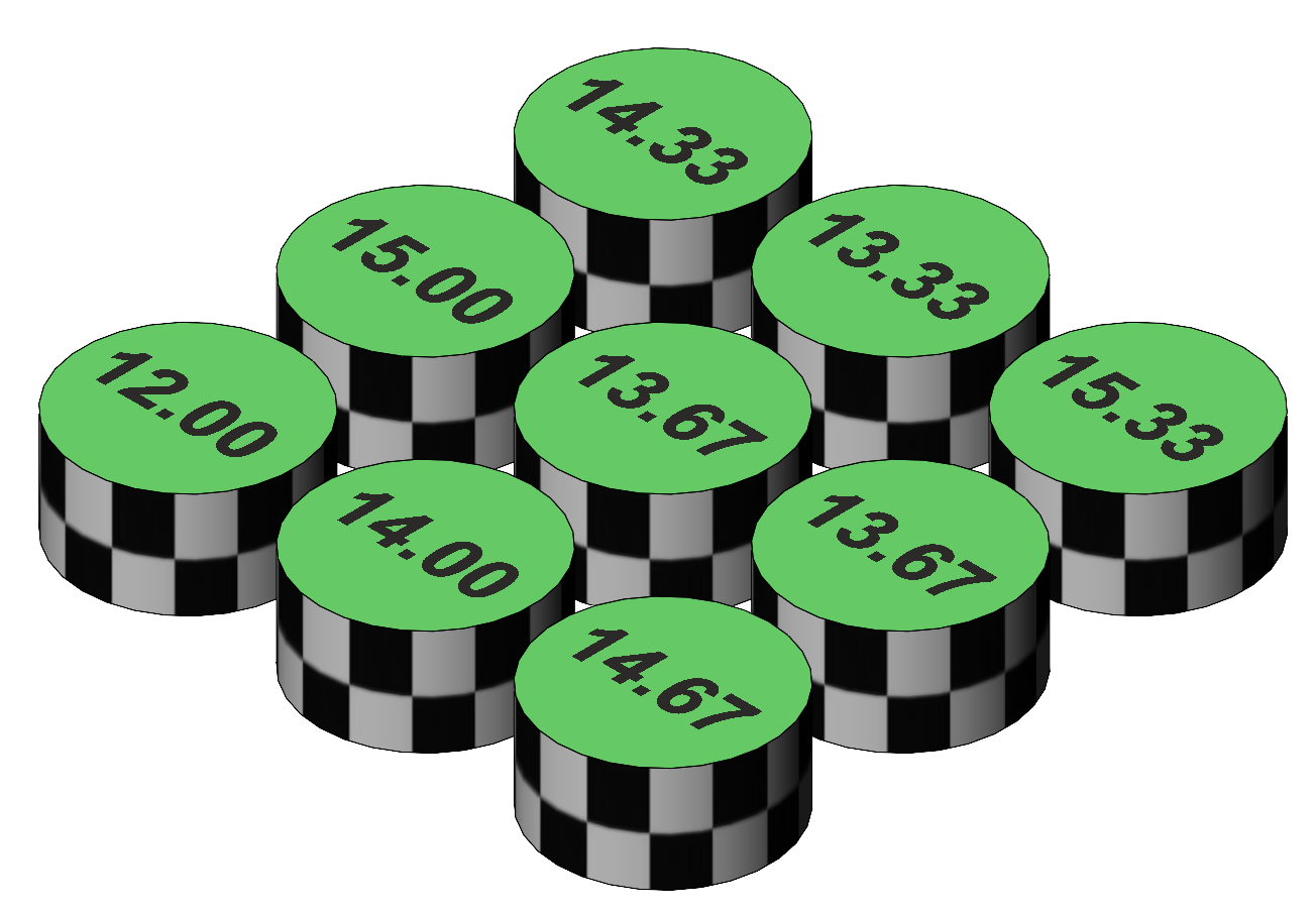
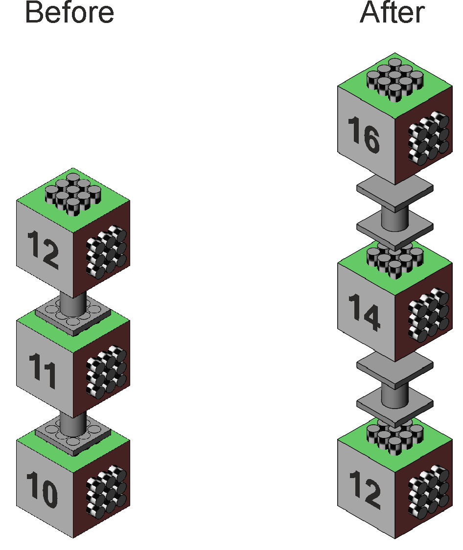
The previous page dealt with Two way rep meas on one factor. Two-way anova, repeated measures on both factorsA group of 9 subjects each drink a preparation containing amino acids, proteins, and peptides. The drink tastes (and smells) medicinal. A few days later they drink a preparation that tastes medicinal but contains no active ingredients. A few days later again they drink tea. All subjects undertake a memory test before their drink, and then again an hour after their drink. The test scores are shown in Table 1. Notice the repeated measures – the same subjects are tested before and after their drink, and the same subjects receive all 3 drinks. This is a repeated measures design on both factors, sometimes called a "randomised blocks" design. The depiction of the subjects in a given cell of the design shows two sets of projecting tubes. These represent the subject data within each cell which, in the vertical orientation, is averaged over the red factor, and in the horizontal orientation, is averaged over the green factor. The subject scores averaged over the green factor are shown on the left and coloured red. There are three arrays of these subject averages, one for each level of the red factor. Similarly, the subject scores averaged over the red factor are shown on the bottom and coloured green. There are two arrays of these subject averages, one for each level of the green factor. Because these are the same subjects, all six of their scores can be averaged, and this is shown as patterned balls on the lower left of the diagram.
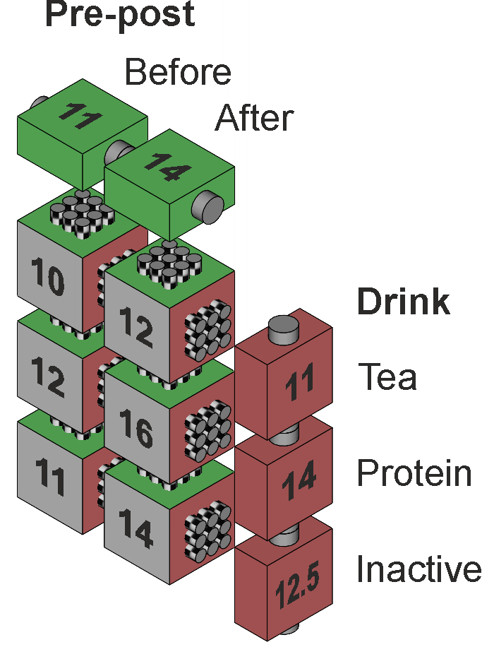
Figure 1. Representation of the two-way anova with repeated measures on both factors. Notice also that numerically the data is the same as that for the previous two-way anovas. Table 1. Memory test scores for 9 subjects, before and after 3 drink types.
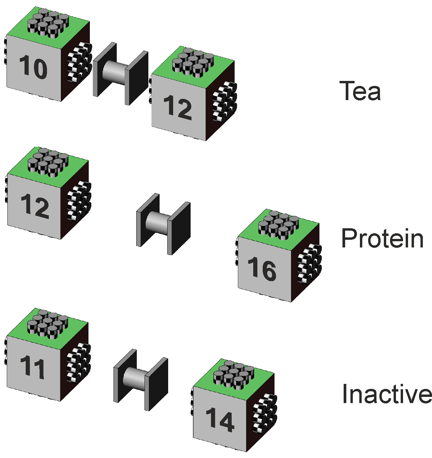
As before, the question here is whether the protein drink improves the memory of the subjects compared to an inactive drink or to tea. The subjects provide their own control data, in that their baseline memory is tested before their drink, so that their test afterwards gives a better picture of whether the drink has any effect. In addition, because the same subjects are used for each drink, the picture of the differences between the drinks should also be clearer. This all works well provided that the subjects do not learn or remember anything from the pre-test that modifies their post-test scores, and provided that the subjects reactions to one drink are not affected by a previous drink or affect their next drink. The expected "better picture" only materialises if the subjects show consistency in their memory scores from Before to After and from drink to drink, that is, their scores are "adequately" correlated. The labels for the factors are "Drink" and "Pre-post", with levels "Tea", "Protein", and "Inactive", and "Before" and "After". The measure is "Memory". The factor and cell means are illustrated in Figure 2.
Figure 2. Factor and cell means. As discussed in the Two way rep meas on one factor page, the question could be answered by calculating change scores for the subjects, both between the Before and After scores and between their Tea, Protein, and Inactive scores, but this brings problems which we have rehearsed in previous pages. Instead we investigate the interaction effect between the Before and After scores and the Tea, Protein, and Inactive scores. The follow-on analyses of main effects (insignificant interaction) or simple main effects (significant interaction) and related pairwise comparisons identify the sources of any differences in more detail.
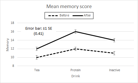
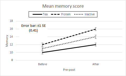
Profile plotsFrom the cell means we draw Pre-post × Drink and Drink × Pre-post profile plots which are the same as for the Two way factorial anova and Two way rep meas on one factor data.
Figure 3. Profile plots of cell means for Pre-post × Drink and Drink × Pre-post. The cell, Drink, and Pre-post means are the same as for both the two-way anovas, as shown in Table 2. As before, the profile plots have the same profiles. Also as before, the ±1 SE error bar of the various cell means is given by s / √n for each cell if their standard deviations are markedly different, or by √(MS(Cells) / n) for each, where MS(Cells) is the average of the cell variances. For our data, we use SE = √ (1.5 / 9) = 0.41 for each cell mean. Table 2. Memory test mean scores for Drink, Pre-post, and Drink × Pre-post.
The Two way rep meas on one factor page provided the general principles of calculating SS, MS, and df for an effect using means. From the previous two-way anovas we have already calculated SS[D], SS[P], and SS[DP] as 81.0, 121.5, and 211.5 while df[D], df[P], and df[DP] are 2, 1, and 5. SS(Drink) = SS[D] = 81.0 with df(Drink) = 2, hence MS(Drink) = 40.5; and SS(Pre-Post) = SS[P] = 121.5 with df(Pre-Post) = 1, hence MS(Pre-Post) = 121.5. The interaction effect SS(Drink×Pre-Post) = SS[DP] – SS(Drink) – SS(Pre-post) = 211.5 – 81.0 – 121.5 = 9, df(Drink×Pre-Post) = df[DP] – df(Drink) – df(Pre-post) = 5 – 2 – 1 = 2, and so MS(Drink×Pre-Post) = SS(Drink×Pre-Post) / df(Drink×Pre-Post) = 9 / 2 = 4.5.
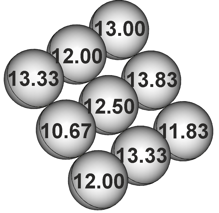
Error varianceWe begin with the calculation of error variation by taking the average variance of the data in each cell, which for our data is (1.5 + 1.5 + 1.5 + 1.5 + 1.5 + 1.5) / 6 = 1.5. The df is the sum of the df for each cell, which for our data is 6 · (n–1) = 4 · 8 = 48. Error variation, expressed as SS, is 48 · 1.5 = 72. For our data, however, the subjects provide memory test scores both before and after their drink. This allows the Before to After difference to give a better picture of whether the drink has any effect, and also allows a better picture of any differences between the drinks. The dependent samples section in the One way anova page shows how to account for the portion of the sample variation that can be attributed to variation between subjects, and how to deduct it from the cells' variation to give the remaining, smaller, variation that is shown within subjects. The between-subjects SS is calculated from the variation shown by the subjects' overall average scores, and is deducted from the cells' error SS to give the within-subjects variation that can also be called residual. Table 3 shows the average subjects' scores, the calculated variance of the average, and the calculated SS given that each average is based upon 6 scores and the df for the subjects is 9 – 1 = 8. Table 3. Memory test mean scores for subjects [S].
Figure 4. Representation of the subjects overall average scores. The SS for Subject is given by the variance of the subject means, [S], 0.97, multiplied by the number of scores used in each mean, 3 · 2 = 6, and multiplied by the df for the variance, n – 1 = 8, to give SS(Between subjects) = 46.33. This is deducted from SS(Error) and df(Error) to yield SS(Residual) = 72 - 46.33 = 27.67 with df(Resid) = 48 - 8 = 40, hence MS(Residual) = 27.67 / 40 = 0.64. We can note that df(Between subjects) = 8, and hence MS(Between subjects) = 46.33 / 8 = 5.79. On the face of it, the repeated measures across both factors has given a much reduced error term, MS(Residual) = 0.64, compared to the error term from the two-way factorial anova with no repeated measures where MS(Error) = 1.5. The "cost" in the loss of degrees of freedom is relatively modest, df(Residual) = 40 compared with df(Error) = 48.
Anova summaryThe results of the calculations are summarised as per Table 4. Table 4. Anova summary.
These numerical results are almost exactly the same as the results seen in the Two way factorial anova and Two way rep meas on one factor pages. Their interpretation is also the same, since the F ratios are all significant. The difference is a smaller error term. The calculation of pairwise comparisons of main effect means, analysis of simple main effects, and calculation of pairwise comparisons of simple main effect means are the same as for the Two way factorial anova, where MS(Residual) is used in place of MS(Error). Note that the error bar SEs of the various cell means shown on the interaction profile plots is given by the square root of MS(Cells) / n for each, where MS(Cells) is the average of the cell variances. For our data, we use SE = √ (1.5 / 9) = 0.41 for each cell mean. This is different from the provision of the error bars on the main effects profile plots, where the SE is based on MS(Residual).
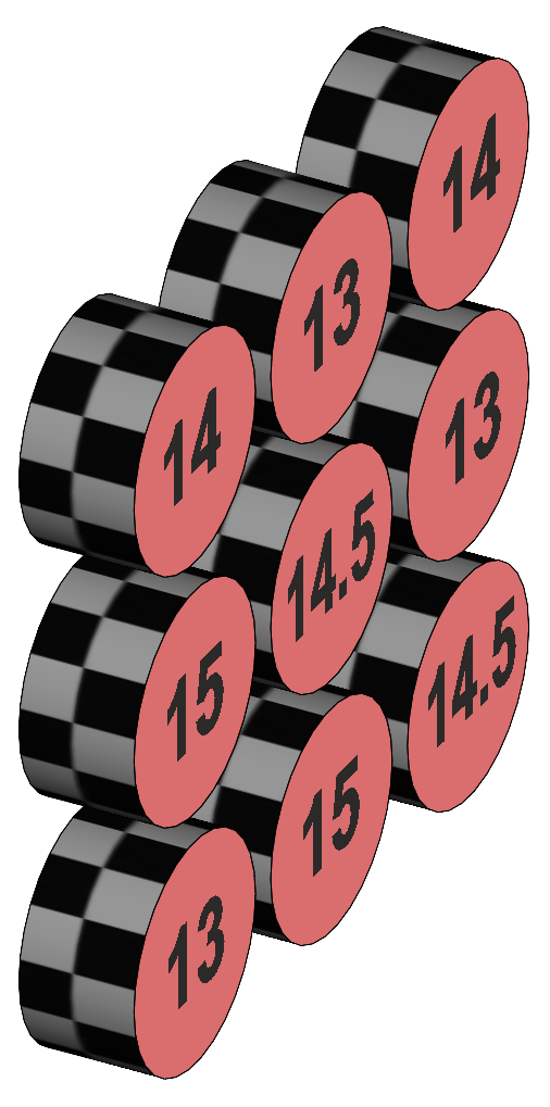
Further analysis of SS(Residual) error varianceAs suggested in Figure 1, there are three sets of subject average scores. One set is as analysed earlier, [S], the subject overall averages illustrated in Figure 4. This set provides the value of SS(Between subjects) which is subtracted from SS(Cells) to yield SS(Residual), also called SS(Within subjects). A second set comprises three arrays, being the subject average scores across Pre-post, one array for each of Tea, Protein, and Inactive. These three are listed as columns in Table 5, labelled [SD], and illustrated as arrays in Figure 5. These scores represent an interaction between the subjects and the Drink factor, Subject × Drink. Table 5. Subject average scores across Before and After for each level of Drink [SD].
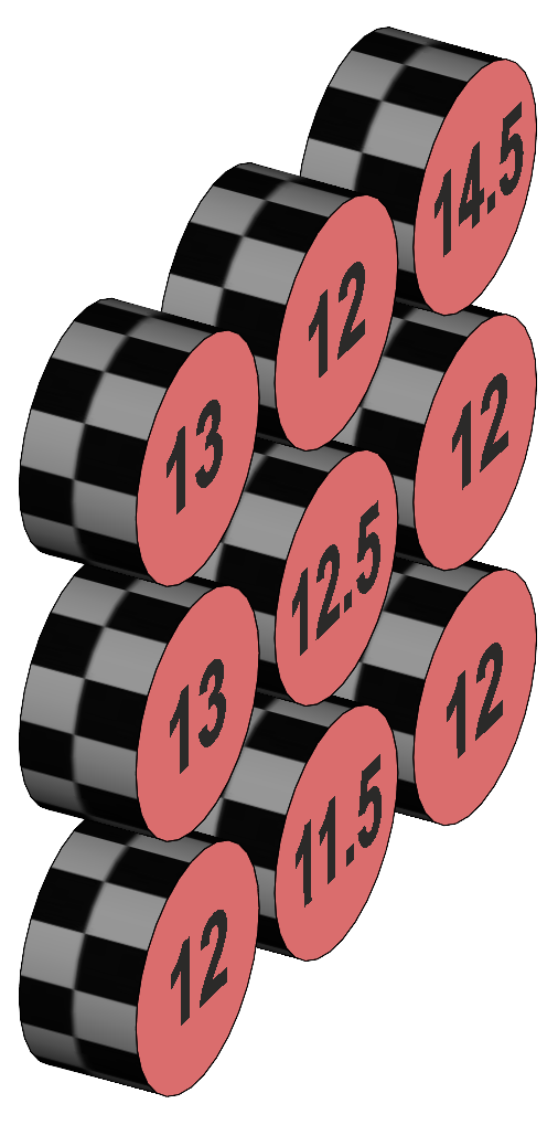
Figure 5. Depiction of the subject scores averaged over Before and After at each level of Drink: Tea, Protein, and Inactive. The table of subject average scores for each level of Drink may be labelled [SD]. SS[SD] is 135. Like any interaction, SS(Subject × Drink) may be calculated by subtracting SS(Subject) and SS(Drink), in this case subtracting 46.33 and 81, from SS[SD]. The result is SS(Subject × Drink) = 7.7. A third set comprises two arrays, being the subject average scores across Drink, one array for each of Before and After. These two are listed as columns in Table 6 and illustrated as arrays in Figure 6. These scores represent an interaction between subjects and the Pre-post factor, Subject × Pre-post. Table 6. Subject average scores across Tea, Protein, and Inactive for each level of Pre-post [SP].
Figure 6. Subject scores averaged over each level of Drink (Tea, Protein, and Inactive) at Before and After. The table of subject average scores for each level of Pre-post may be labelled [SP]. SS[SP] is 174.83. Like any interaction, SS(Subject × Pre-post) may be calculated by subtracting SS(Subject) and SS(Pre-post), in this case subtracting 46.33 and 121.5 from SS[SP]. The result is SS(Subject × Pre-post) = 7.0. It is possible to partition the residual error variation, SS(Resid), into three error terms. We consider SS(Resid) as the pooling of the interaction effects between subjects and the factors, specifically the interaction of subjects with Drink, Pre-post, and Drink × Pre-post. We have calculated SS(Subject × Drink) and SS(Subject × Pre-post) . Subtracting them from SS(Resid) leaves a "residual" from SS(Resid) which is SS(Subject × Drink × Pre-post). These various interactions with subjects can be used as error terms to test their corresponding effects: Drink is tested against Subject × Drink; Pre-post is tested against Subject × Pre-post; and Drink × Pre-post is tested against Subject × Drink × Pre-post. These are listed in Table 7. Table 7. Tests of factor effects with partitioned residual error variance.
These error terms are used by SPSS in its analysis of repeated measures on both factors. Unless the data has ample degrees of freedom, the loss of power may not be compensated by the increased precision in the test of each of the factor effects. MS(Residual) may be a better error term for testing the factor effects, and can be constructed from the SPSS results table by pooling the SS and df of the separate error terms. For example, Table 8 shows the value of these error terms for our data. Table 8. Partitioned residual error variance.
Note that SS(Subject×Drink) + SS(Subject×Pre-post) + SS(Subject×Drink×Pre-post) = 7.7 + 7.0 + 11.0 = 27.7 = SS(Residual), and similarly for the degrees of freedom. For our data, MS(Residual) = 0.64 with df = 40. Only the test of the Drink factor potentially benefits from the partition with a lower test MS = 0.48. The tests of Pre-post and the interaction suffer, not only from a larger test MS but smaller degrees of freedom. This is an inevitable and general outcome of partitioning, illustrated in Table 9 which shows the lower critical F values for each test when using MS(Residual) as the pooled error term. Table 9. Critical F for effect tests.
Pairwise comparisons following significant main effectsFollowing an insignificant interaction, the main effects may be examined and, if significant, analysed further using pairwise comparisons. The issue in pairwise comparisons for repeated measures data is the correct choice of the standard error in the t-tests. The choice of the error term to use in constructing SEdiff for pairwise comparisons for a given factor follows the error term used for the main effect. Because both Drink and Pre-post are within subjects factors, SEdiff is based upon MS(Resid) for both factors. Note that SPSS uses MS(Subject×Drink) for Drink main effect comparisons and MS(Subject×Pre-post) for Pre-post main effect comparisons. For the current data, SEdiff = √ (2 · 0.64 / 18) = 0.27 for comparisons between Tea, Protein, and Inactive main effect means because each mean is based upon 18 scores, and SEdiff = √ (2 · 0.64 / 27) = 0.22 for the comparison between the Before and After main effect means because each mean is based upon 27 scores.
Simple main effects in repeated measures on two factorsFollowing a significant interaction, there are two sets of simple main effects, one for each factor which corresponds to one of the interaction profile plots. Both sets of simple main effects are constructed following a significant interaction effect. One set examines the simple main effects of Pre-post for each of the three drinks separately, and one set examines the simple main effects of Drink for each of the Pre-post levels of Before and After separately. The simple main effects of Pre-post for Tea are given by a one-way anova of the Before and After means for Tea, being 10 and 12; for the Protein means 12 and 16; and for the Inactive means of 11 and 14. The required error term for the simple main effects of Pre-post is MS(Residual) from Table 4. The F ratio degrees of freedom are 1 and 40, being the df for the simple effect (two means, df = 2 – 1 = 1) and the df for MS(Residual) of 40. We remember that the MS of an effect is given by multiplying the variance of its means by the number of data items which make up each mean, here 9. The summary table of the simple main effects for Pre-post is shown in Table 10. Table 10. Simple main effects for Pre-post.
All three simple main effects of Pre-post are significant, suggesting that the Tea, Protein, and Inactive drinks each show a difference from Before to After. Because there are only two levels of the Pre-post factor, the actual nature of the difference is immediately given by inspecting the interaction profile plots or the table of cell means, where we see that, for each drink, the After mean is significantly higher than the Before mean. Each drink seems to result in a significant increase in the memory test scores of our subjects. If this factor comprised three or more levels, the follow-on is to conduct "simple" pairwise comparisons for each simple main effect. As a check, adding up the SS for the Pre-post simple main effects gives 18 + 72 + 40.5 = 130.5, which is the value given by adding up SS(Pre-post) and SS(Interaction) = 121.5 + 9 = 130.5. The simple main effects of Drink for each level of Pre-post are given by a one-way anova of the Before means of Tea, Protein, and Inactive, being 10, 12, and 11, and a second one-way anova of the After means, 12, 16, and 14. The appropriate error term is MS(Resid). We remember that the MS of an effect is given by multiplying the variance of its means by the number of data items which make up each mean, here 9. The summary table of the simple main effects for Drink is shown in Table 11. Table 11. Simple main effects for Drink.
The two simple main effects of Drink are significant, suggesting that the Tea, Protein, and Inactive drinks show a significant difference in their Before means, p <.001, and also show a significant difference in their After means, p <.001. This suggests that the drink groups have different baseline (Before) memory scores. At the least, we can say that the highest Before mean is significantly different from the lowest Before mean — that the Tea Before mean of 10 is significantly lower than the Protein Before mean of 12. We need pairwise comparisons to tells us whether the Tea Before mean is different from the Inactive Before mean, and whether the Protein Before mean is different from the Inactive Before mean. The second result is probably the one we hope for as the investigator, telling us that the After means are significantly different. At the least we can say that the highest After mean is significantly different from the lowest After mean — that the Tea After mean of 12 is significantly lower than the Protein After mean of 16 — and that pairwise comparisons are needed to tell us about the other After mean differences. Adding up the variation, that is the SS, for the Drink simple main effects gives 18 + 72 = 90, and similarly the total df is 2 + 2 = 4. We can see that these are the values given by adding up SS(Drink) and SS(Interaction) = 81 + 9 = 90 and df(Drink) and df(Interaction) = 2 + 2 = 4.
"Simple" pairwise comparisons following significant simple main effectsThe issue in pairwise comparisons for repeated measures data is the correct choice of the standard error in the t-tests. We refer to the choices made in the analysis of the simple main effects, and continue with those choices for "simple" pairwise comparisons. From Table 11, the simple main effects anova shows a significant simple main effect for the Drink factor at Pre-post = Before. We compare the mean Protein Before memory score with the mean Inactive Before and Tea Before means, and the mean Inactive Before with Tea Before. We remember that conducting separate significance tests, 3 for each family in this case, inflates the family-wise Type I error rate; that simple LSD t-tests are acceptable given no more that 3 means being compared; and that Sidak or Tukey tests or corrections are otherwise indicated. A t-test for the difference between two cell means uses SEdiff calculated as √ (2 · MS / 9), where the value of MS is given by that used in the test of the parent simple main effect and the value of "9" is the cell n. Table 11 shows that MS(Resid) is used to test the Drink simple main effects, and hence the pairwise comparisons use MS(Resid) as the basis of the SEdiff to test difference between drinks at each level of Pre-post, that is, Before and After. MS(Resid) = 0.64 hence SEdiff = √ (2 · 0.64 / 9) = 0.38. The df for the t-test are as for MS(Resid), 40. For the difference between Tea and Inactive when Pre-post is Before we have t = (10 – 11) / 0.38 = –2.65, p = .01; between Inactive and Protein we have t = (11 – 12) / 0.38 = –2.65, p = .01; and between Tea and Protein we have t = (10 – 12) / 0.38 = –5.3, p < .001. For the Before means, all the difference between drinks are significant. While the Drink × Pre-post profile plot shows relatively small gaps between the Before Drink means, these are revealed to be significant with the repeated measures analysis on the Drink factor. Following the significant simple main effect for the Drink factor at Pre-post = After, we compare the mean Protein After memory score with the mean Inactive After and Tea After scores, and the mean Inactive After with Tea After. For the comparison between Tea and Inactive when Pre-post is After we have t = (12 – 14) / 0.38 = –5.3, p < .001; between Inactive and Protein we have t = (14 – 16) / 0.38 = –5.3, p < .001; and between Tea and Protein we have t = (12 – 16) / 0.38 = –10.59, p < .001. We see that, for the After means, all the differences between Drink are significant. A check with the Drink × Pre-post profile plot shows the relatively large gaps between the After Drink means, consistent with the pairwise comparisons. Figure 7 illustrates the "simple" pairwise comparisons between the Drink means at Pre-post = Before, and between the Drink means at Pre-post = After. The cells have been ordered according to their means. Note that the comparisons are within subjects, that is, the subject tubes connect from one cell mean to another. This signifies that SEdiff for these comparisons is based upon MS(Resid).
Figure 7. Depiction of pairwise comparisons between
Drink at each level of Pre-post, differences relative to 2·SEdiff.
From Table 10, the simple main effects anovas for the Pre-post factor show a significant simple main effect for each of Pre-post for Tea, Protein, and Inactive drinks. We can compare the mean Tea Before memory score with the mean Tea After, and so on for the Protein and Inactive drinks. We calculate a pairwise comparison for the Tea means in order to illustrate the general principles. We note that these pairwise comparisons are not necessary; if there is a significant simple main effect for a factor with two levels it is immediately clear from the profile plot or the cell means which mean is significantly higher than which other. We see that MS(Residual) is used to test the Pre-post simple main effects, and hence the Pre-post pairwise comparisons use MS(Residual). MS(Residual) = 0.64 hence SE = √ (2 · 0.64 / 9) = 0.38. We note the division by 9 because each cell mean is based upon 9 scores. The df for the t-test are as for MS(Residual), 40. For the comparison between Tea Before and Tea After we have t = (10 – 12) / 0.38 = –5.30, p <.001. We remember that t2(df) = F(1,df) and see that –4.92 = 28 = F from Table 10 as expected. Figure 8 illustrates the "simple" pairwise comparisons between Before and After at each level of Drink. Note the alignment of the subject tubes connecting Before to After, signifying that the comparisons are within subjects and hence that SEdiff is based on MS(Residual).
Figure 8. Depiction of pairwise comparisons between Pre-post at each level of Drink, differences relative to 2·SEdiff. Note the same subjects in each cell being compared, hence SEdiff uses MS(Resid). From the repeated measures section of the One way anova page we may remember the availability of specific pairwise comparisons which use the correlation between the pairs of factor levels involved. The technique is available for the two-way repeated measures design for pairwise and "simple" pairwise comparisons between main effect or simple main effect means of a within-subjects factor with more than 2 levels. We do not rehearse their application here, but mention them because some statistical analysis software packages, such as SPSS, apply these specific tests, and their results may not agree with the results expected for a more general test which uses the average correlation, equivalent to using unadjusted MS(Residual).
SummaryThe analysis of the two-way anova with repeated measures on two factors follows the same procedures as the two-way factorial anova in the calculation of main and interaction SS, df, and MS. The difference is that the design allows the separation of within and between subjects' error variation. The issue in the repeated measures anova is the choice of the correct error MS for the main and interaction effects and for the simple main effects, and the choice of the correct SEdiff in the pairwise comparisons t-tests following significant main effects or significant simple main effects. The between-subjects error variation may be called SS(Subject) and the within-subjects error variation may be called SS(Residual) to remind us how they are calculated. SS(Subj) is the variation seen in the overall mean scores of the subjects and is subtracted from the variation seen in the cells, SS(Cells), to give SS(Resid). Similarly, the degrees of freedom for the subjects, df(Subj), is subtracted from df(Cells) to give df(Resid). Hence MS(Subj) = SS(Subj)/df(Subj) and MS(Resid) = SS(Resid)/df(Resid). Other authors call between-subjects and within-subjects error variation by other terms when they are calculated by other, more mathematically efficient, ways or when they occur in different domains. Given an insignificant interaction, significant main effects may be analysed further using pairwise comparisons. The appropriate SEdiff for the t-tests of differences between Factor A or B main effect means is based on MS(Resid) since both factors are within subjects. Given a significant interaction, testing the simple main effects of either factor uses MS(Resid). A significant simple main effect may be analysed further using pairwise comparisons. The appropriate SEdiff for the t-tests for differences between both factor simple main effect means is based on MS(Resid). Note that SPSS uses different error terms for simple main effects and for simple pairwise comparisons which are based as required upon SS(Subject), SS(Resid), SS(Subject × Factor A), SS(Subject × Factor B), and SS(Subject × Factor A × Factor B) and their pools. The next page deals with the Three-way Anova.
| ||||||||||||||||||||||||||||||||||||||||||||||||||||||||||||||||||||||||||||||||||||||||||||||||||||||||||||||||||||||||||||||||||||||||||||||||||||||||||||||||||||||||||||||||||||||||||||||||||||||||||||||||||||||||||||||||||||||||||||||||||||||||||||||||||||||||||||||||||||||||||||||||||||||||||||||||||||||||||||||||||||||||||||||||||||||||||||||||||||||||||||||||||||||||||||||||||||||||||||||||||||||||||||||||||||||||||||||||||||||||||||||||||||||||||||||||||||||||||||||||||||||||||||||||||||||||||||||||||||||||||||||||||||||||||||||||||||
|
©2025 Lester Gilbert |