![]()
![]()
![]()
![]()
![]()
![]()
![]()
|
|
|
Introduction to interactionWe begin with some terminology (variable, factor, factor level, effect, interaction) and a way of talking about our data and its analysis. A "variable" is something we measure, such as a person's score on a test of dexterity. We could also say that whether a student is studying art or mathematics is something we 'measure' and call it a variable, but that is a little awkward because a subject of study isn't usually said to be something that is 'measured', it is a given. In general, we will call a 'given measure' a "factor" in our discussion. A factor has two or more "levels", so one level of the Study Subject factor is Maths, and the other level of the Study Subject factor is Art. We might investigate the effect of Study Subject on Dexterity. The "effect" of a factor is the difference between the levels of the factor in a variable of interest, for example the difference in Dexterity between Maths and Arts students. We note that the difference is given by the difference between the mean Dexterity scores of the Maths students and the mean Dexterity scores of the Arts students. The mean is the technically correct term for what we would otherwise call the average. We might have read about the influence of caffeine on hand-eye coordination, and we might wonder if a drink of strong coffee might improve (or reduce) dexterity. As a good experimenter, we know that we should test caffeine against a control or neutral drink such as water, giving us a Drink factor with two levels (Caffeine and Water). Finally, we wonder, for some reason, whether Maths students might show more of an increase in dexterity than Arts students following a drink of coffee. We are wondering whether there is an "interaction" between the factors of Study Subject and Drink. Example dataWe imagine that we have asked 18 of our Maths friends, and 18 of our Arts friends, to join us for drinks. Half are given a glass of water, half a mug of coffee, and after 20 minutes of discussion about the ways of the world they all take a test of Dexterity which yields a score between 0 and 100. The raw data are not very interesting, the summary descriptive statistics are, as presented in Table 1 below. Table 1. Descriptive statistics
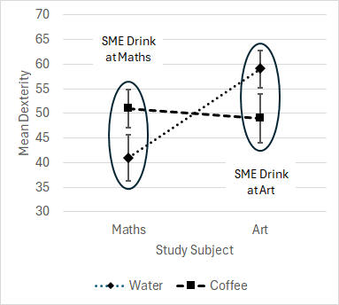
InteractionIn our example, we might consider that Arts students might (or might not) have a higher mean Dexterity score than Maths students. We might consider that a drink of coffee might (or might not) lead to a higher mean Dexterity score than a drink of water. Regardless of either of these considerations, interaction is where Drink has a differential effect on Dexterity depending on whether the students are studying Maths or Art. Equivalently, interaction is where Study Subject has a differential effect on Dexterity depending on whether the Drink is Coffee or Water. Visualizing interactionThere is no substitute for profile plots (also called trend graphs). Always prepare the two relevant profile plots when attempting to understand or interpret the interaction between two factors. The plots are of the mean of the variable with one of the factors on the plot X-axis and the other factor being the plot lines. It is also very useful for each mean to be shown with an error bar which is plus and minus 1 standard error (±1SE), as shown in Figure 1.
Figure 1. Profile plots Note the completely different picture given by each profile plot. One or other plot may give a preferred picture of the data, but both are essential to start with. We may remember the rule of thumb that two means which are more than 2 SEs apart are probably significantly different -- that is, if each is plotted with a ±1SE error bar, the bars do not overlap. The first profile plot shows that there may or may not be a significant difference in mean Dexterity (the error bars are barely separate) after drinking either Water or Coffee for Maths students and for Art students. On the other hand, the second profile plot shows what we might have missed -- there seems to be a highly significant difference in mean Dexterity after drinking Water between Maths and Art students (the error bars clearly are well separated and do not overlap), but there is certainly not a significant difference after drinking coffee between Maths and Arts students (the error bars do overlap). Interpreting the profile plotInteraction is shown when the profiles (plot lines) are not parallel. Another way of saying this is that the profiles show different or divergent trends. Of course, random sampling variation means that profiles will never be perfectly parallel, and some degree of non-parallelism is usually present in any plot. The error bars guide you when deciding whether any divergence between profiles is likely to be significant. Please note that interaction is NOT shown by profile lines crossing over each other. This is a common misconception that can be found in various semi-expert web pages and discussion groups. It is the divergence of trend and non-parallelism, and not the crossing, of profile lines which signals interaction. The size of an interaction effectThe interaction effect between two factors is what is left after accounting for the trends or main effects of each factor considered separately. We begin by summarising our data so far. Table 2 shows the cell means, the factor means, and the grand mean. Table 2. Cell, factor, and grand means
Looking at Drink, the overall mean Dexterity score of the students who drank Water is 50. Since the grand mean is 50, the effect of Water on Dexterity is 0. Similarly, the overall mean Dexterity score of the students who drank Coffee is 50, and so the effect of Coffee on Dexterity is 0. The technical definition of "effect" is the difference between the mean in question and the grand mean (other things being equal, we'll see about that in a moment). The main effect of Water is 0, and the main effect of Coffee is 0. Looking at Study Subject, the overall mean Dexterity score of Maths students is 46. The grand mean is 50 and so the effect of Maths is -4. Similarly, the overall mean Dexterity score of the Art students is 54, and so the effect of Art is +4. These are summarised in Table 3. Table 3. Main effects
Table 4 shows the cell means that would be expected if there was no interaction between Drink and Study Subject. The logic runs as follows. With no interaction, the cell mean for Maths and Water is expected to be the grand mean plus the Maths effect plus the Water effect, 50 + -4 + 0 = 46. With no interaction, the cell mean for Art and Coffee is expected to be the grand mean plus the Art effect plus the Coffee effect, 50 + 4 + 0 = 54. And so on for the other cells. Table 4. Expected cell means if there is no interaction
Table 5 shows the differences between the observed call means and the cell means that would be expected if there was no interaction between the factors. These differences are the interaction effects. Table 5. Difference between observed and expected cell means if there is no interaction
The interaction effects are -5, 5, 5, and -5. If there was no interaction, these differences would be 0, 0, 0, and 0. Another way of looking at main and interaction effects is to examine the differences between the observed cell means and the grand mean, as shown in Table 6. We can call these differences the cell effects. Table 6. Difference between observed cell means and the grand mean
The cell effects are -9, 9, 1, and -1. We know these must consist of the total of the two main effects and the interaction effect for a given cell. In order to establish the interaction effect itself we need to subtract the main effects from the cell effect to see what is left. For example, the cell effect for Maths and Water is -9, so subtracting the Maths effect, -4, and subtracting the Water effect, 0, gives -9 - -4 - 0 = -5, which is the interaction effect for Maths and Water as seen in Table 5. The cell effect for Art and Coffee is -1, minus the Art effect, +4, minus the Coffee effect, 0, giving -1 - 4 - 0 = -5. And so on for the other cells. Computing the significance of an interaction effectWe might say that the main effects of the Study Subject factor are -4 and +4, but that isn't quite right, since it is the main effect of Art which is +4 and the main effect of Maths which is -4. Instead, technically, the main effects of a factor is given by the variation shown by its effects. Similarly, we might say that the interaction effects of Study Subject × Drink are -5, 5, 5, and -5, but again, technically, the interaction effect is given by the variation shown by these effects. The necessary calculations for main and interaction effects are explained in some detail the page on the One way anova and in the page on the Two independent samples anova. The calculation of significance compares the MS(Effect) with MS(Error). The anova summary table for the example data is given in Table 7. Table 7. Anova summary table
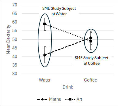
Simple main effects following a significant interaction effectTests of significance always start with the interaction effects. If the interaction is significant, main effects are not examined. In our example, the Drink × Study Subject interaction is significant, and so we disregard the Drink and Study Subject main effects (which happen to be non-significant). Instead, attention moves on to the analysis of simple main effects. This is because the finding of a significant interaction is a finding that the effects of one factor depend on a particular level of the other and cannot be generalised to all the levels. (We explore the merits of this claim below, after considering simple main effects.) A simple main effect is the effect of a factor at a particular level of the other factor. In our example, we would consider the simple main effect of Drink -- the difference in mean Dexterity between Water and Coffee -- for Maths students, and the simple main effect of Drink for Art students. Similarly, we continue by considering the simple main effect of Study Subject -- the difference in mean Dexterity between Maths and Art students -- after a drink of Water, and the simple main effect of Study Subject after a drink of Coffee. Figure 2 shows the best way of inspecting the profile plots to discern the SMEs and whether they are likely to be significant. The key idea is that overlap or otherwise of the error bars is most easily seen when they are stacked vertically, rather than trying to read along a plot line to see if the error bars at each end overlap.
Figure 2. Inspecting the profile plots for the likely significance of SMEs For the example data, there may or may not be a significant SME of Drink at Maths or at Art (the error bars are barely separate), while it seems visually clear that there is a significant SME of Study Subject at Water (the error bars clearly do not overlap and are well separated) and a non-significant SME of Study Subject at Coffee (the error bars overlap). These visual impressions require formal tests of significance as explained in the page on the Two independent samples anova. Interpreting main effects given significant interactionAn ongoing debate in various semi-expert web pages and discussion groups concerns the status and meaning of a main effect, whether significant or otherwise, in the context of a significant interaction. We may explore this issue by considering three examples, where the interaction effect is significant but no, one, or both main effects are significant. In these examples, the interaction effects are -5, 5, 5, and -5 as seen earlier, MS(Drink × Study Subject) = 900, F(1,32) = 5.21, p = 0.03* (* significant at the 0.05 level). The main effects are -2 and 2 when not significant, MS(non-sig ME) = 144, F(1,32) = 0.83, p = .37 (ns), or are -10 and 10 when significant, MS(sig ME) = 3600, F(1,32) = 20.84, p < .001 (off the scale!). Significant interaction, no significant main effects | |||||||||||||||||||||||||||||||||||||||||||||||||||||||||||||||||||||||||||||||||||||||||||||||||||||||||||||||||||||||||||||||||||||||||||||||||||||||||||||||||||||||||||||||||||||||||||||||||||||||||||||||||||||||||||||||||||||||||||||||||||||||||||||||||||||||||||||||||||||||||||||||||||||||||||||||||||||||||||||||||||||||||||||||||||||||||||||||||||||||||||||||||||||||||||||||||||||||||||||||||||||||||||||||||||||||||||||||||||||||||||||||||||||||||||||||||||||||||||||||||||||||||||||||||||||||||||||||||||||||||||||||||||||||||||||||||||||||||||||||||||||||||||||||||||||||||||||
| Source | SS | df | MS | F | p |
| Drink | 144 | 1 | 144 | 0.83 | 0.368 |
| Study Subject | 144 | 1 | 144 | 0.83 | 0.368 |
| Drink × Study Subject | 900 | 1 | 900 | 5.21 | 0.029 |
| Error | 5528 | 32 | 172.75 |
The interaction effect is significant. We know not to interpret the main effects given a significant interaction, but human nature being what it is, we sneak a peek and see completely non-significant Drink and Study Subject effects, so think that, yeah, neither Water nor Coffee affected Dexterity much, and the Maths and Art students were not much different on Dexterity. Then, like the Professor said, we run the analyses of simple main effects.
| Source | SS | df | MS | F | p | ||
| SME Drink at Maths | 882 | 1 | 882 | 5.11 | 0.031 | ||
| SME Drink at Art | 162 | 1 | 162 | 0.94 | 0.340 | ||
| SME Study Subj at Water | 882 | 1 | 882 | 5.11 | 0.031 | ||
| SME Study Subj at Coffee | 162 | 1 | 162 | 0.94 | 0.340 | ||
| Error | 5528 | 32 | 172.75 | ||||
The simple main effect (SME) of Drink at Maths is significant, meaning that the mean Dexterity score for the Maths students is significantly different depending on whether they drank Water or Coffee. Oh. Wait ... didn't we just think that there was no significant Drink effect from our sneak peek? We inspect the profile plots and see that it is the mean Dexterity after Coffee which is significantly higher than after Water for the Maths students. OK, makes sense, interesting.
We move along and find the SME of Drink at Art is not significant, meaning that the mean Dexterity score for the Art students is not significantly different depending on whether they drank Water or Coffee. Oh again. We inspect the profile plots and see that the error bars for Coffee and Water overlap, and therefore the small difference that we do see is of no consequence.
Then we see that the SME of Study Subject at Water is significant, meaning that the mean Dexterity score for the Maths students is significantly different from the Art students after drinking Water. Oh, er, again. Wait ... didn't we just think that there was no significant Study Subject effect from our sneak peek, that the Maths and Art students were not much different on Dexterity? We inspect the profile plots and see that it is the mean Dexterity of the Art students which is significantly higher than the Maths students after drinking Water. OK, hmmm, the Art students are more dexterous. Interesting.
And finally we see that the SME of Study Subject at Coffee is not significant, meaning that the mean Dexterity score for the Maths students is not significantly different from the Art students after drinking Coffee. Huh. We inspect the profile plots and see that the mean Dexterity error bar of the Art students overlaps with the Maths students error bar after drinking Coffee. OK, we have a result! The Maths students are as dexterous as the Art students but only after drinking Coffee.
What have we learned? Not to interpret the main effects given a significant interaction, because otherwise we will mislead ourselves.
| Source | SS | df | MS | F | p |
| Drink | 144 | 1 | 144 | 0.83 | 0.368 |
| Study Subject | 3600 | 1 | 3600 | 20.84 | <.001 |
| Drink × Study Subject | 900 | 1 | 900 | 5.21 | 0.029 |
| Error | 5528 | 32 | 172.75 |
The interaction effect is significant. We know not to interpret the main effects given a significant interaction, but human nature being what it is, we sneak a peek and see completely non-significant Drink effect, so think that, yeah, neither Water nor Coffee affected Dexterity much, and an off-the-scale Study Subject effect, so think that the Art students are much more dexterous, which is completely expected, really. Like the Professor said to do, we run the analyses of simple main effects but don't expect to find much because it all looks much like we might have expected.
| Source | SS | df | MS | F | p | ||
| SME Drink at Maths | 882 | 1 | 882 | 5.11 | 0.031 | ||
| SME Drink at Art | 162 | 1 | 162 | 0.94 | 0.340 | ||
| SME Study Subj at Water | 4050 | 1 | 4050 | 23.44 | <.001 | ||
| SME Study Subj at Coffee | 450 | 1 | 450 | 2.60 | 0.116 | ||
| Error | 5528 | 32 | 172.75 | ||||
The SME of Drink at Maths is significant, meaning that the mean Dexterity score for the Maths students is significantly different depending on whether they drank Water or Coffee. Oh. Wait ... didn't we just think that there was no significant Drink effect from our sneak peek? We inspect the profile plots and see that it is the mean Dexterity after Coffee which is significantly higher than after Water for the Maths students. OK, makes sense, interesting.
We move along and find the SME of Drink at Art is not significant, meaning that the mean Dexterity score for the Art students is not significantly different depending on whether they drank Water or Coffee. We inspect the profile plots and see that the error bars for Coffee and Water overlap, and therefore the small difference that we do see is of no consequence.
Then we see that the SME of Study Subject at Water is off-the-scale significant, meaning that the mean Dexterity score for the Maths students is significantly different from the Art students after drinking Water. Well, our sneak peek did have us thinking that the Maths and Art students were different on Dexterity. We inspect the profile plots and see that it is the mean Dexterity of the Art students which is significantly higher than the Maths students after drinking Water. OK, hmmm, the Art students are more dexterous. Not unexpected.
And finally we see that the SME of Study Subject at Coffee is not significant, meaning that the mean Dexterity score for the Maths students is not significantly different from the Art students after drinking Coffee. Oh, er, again.... Didn't we think earlier that there was a significant Study Subject effect from our sneak peek, that the Maths and Art students were quite different on Dexterity? We inspect the profile plots and see that, while the mean Dexterity error bar of the Art students is just separate from the Maths students error bar after drinking Coffee, this is not significant. OK, again we have a result! The Maths students are as dexterous as the Art students after Coffee despite the off-the-scale significance of the Study Subject main effect.
What have we learned? Not to interpret the main effects given a significant interaction, we will mislead ourselves.
| Source | SS | df | MS | F | p |
| Drink | 3600 | 1 | 3600 | 20.84 | <.001 |
| Study Subject | 3600 | 1 | 3600 | 20.84 | <.001 |
| Drink × Study Subject | 900 | 1 | 900 | 5.21 | 0.029 |
| Error | 5528 | 32 | 172.75 |
The interaction effect is significant. I hope we have learned by now not to interpret the main effects given a significant interaction, but human nature being what it is, we sneak a peek and see an off-the-scale significant Drink effect, so think that, yeah, Coffee must boost Dexterity hugely, and an off-the-scale Study Subject effect, so think that the Art students are much more dexterous, both of which are a completely expected results. Do we really need to do like the Professor said, must we run the analyses of simple main effects because that interaction showed just a modest significance, only one star * significant, how could that change those off-the-scale triple-star *** significant main effects? Buckle up....
| Source | SS | df | MS | F | p | ||
| SME Drink at Maths | 4050 | 1 | 4050 | 23.44 | <.001 | ||
| SME Drink at Art | 450 | 1 | 450 | 2.60 | 0.116 | ||
| SME Study Subj at Water | 4050 | 1 | 4050 | 23.44 | <.001 | ||
| SME Study Subj at Coffee | 450 | 1 | 450 | 2.60 | 0.116 | ||
| Error | 5528 | 32 | 172.75 | ||||
The SME of Drink at Maths is significant, meaning that the mean Dexterity score for the Maths students is significantly different depending on whether they drank Water or Coffee. Yes, we were expecting a significant Drink effect from our sneak peek. We inspect the profile plots and see that it is the mean Dexterity after Coffee which is significantly higher than after Water for the Maths students. Yes, we know don't we, Coffee boosts Dexterity.
We move along and find the SME of Drink at Art is not significant, meaning that the mean Dexterity score for the Art students is not significantly different depending on whether they drank Water or Coffee. Wait!!! The significant Drink main effect was off the scale. We inspect the profile plots and see that while the error bars for Coffee and Water do not overlap, they are not sufficiently well separated to denote significance, and therefore the small difference that we do see is of no consequence. Really? Coffee did not boost Dexterity for Art students.
Then we see that the SME of Study Subject at Water is off-the-scale significant, meaning that the mean Dexterity score for the Maths students is significantly different from the Art students after drinking Water. Well, our sneak peek did have us thinking that the Maths and Art students were different on Dexterity. We inspect the profile plots and see that it is the mean Dexterity of the Art students which is significantly higher than the Maths students after drinking Water. OK, hmmm, the Art students are more dexterous. Not unexpected.
And finally we see that the SME of Study Subject at Coffee is not significant, meaning that the mean Dexterity score for the Maths students is not significantly different from the Art students after drinking Coffee. Groan. We inspect the profile plots and see that, while the mean Dexterity error bar of the Art students is only just separate from the Maths students error bar after drinking Coffee, this is not significant. Well, at least we have a result! The Maths students are as dexterous as the Art students after Coffee despite the off-the-scale significance of the Study Subject main effect.
What have we learned? Not to interpret the main effects given a significant interaction, we will mislead ourselves? Was that mentioned earlier? Yeah, a couple of times.
Two things. The good news is that we may now interpret the main effects, and if they are significant we know what to do by way of pairwise comparisons to see which factor level was significantly different from which other level (see the pages on the One way anova and the Two independent samples anova).
The not so good news is that we must now ignore everything we saw from the earlier profile plots. They illustrate plot lines and trends which are not significantly divergent. Despite their visual appearances and looking divergent, that is due to random sampling error, the plot lines are essentially parallel. We must now construct single-line profile plots of the means of the main effects. Here is some sample data with an insignificant interaction but significant main effects, along with their main effect means and their standard error calculated from MS(Error).
| Study Subject | ||||
| Maths | Art | Mean | ||
| Drink | Water | 32 | 56 | 44 |
| Coffee | 48 | 64 | 56 | |
| Mean | 40 | 60 | ||
| Source | SS | df | MS | F | p |
| Drink | 1296 | 1 | 1296 | 7.50 | 0.010 |
| Study Subject | 3600 | 1 | 3600 | 20.84 | <.001 |
| Drink × Study Subject | 144 | 1 | 144 | 0.83 | 0.368 |
| Error | 5528 | 32 | 172.75 |
The Drink main effect is significant. Because there are only two levels of the factor, it is only necessary to inspect the profile plot to state that it is the mean Dexterity score of students who drank Coffee which is significantly higher than those who drank Water. Because the interaction is not significant, this finding applies to both Maths and Art students alike. The Study Subject main effect is significant. Inspection of the profile plot shows that the mean Dexterity score of Art students is significantly higher than Maths. Because the interaction is not significant, this finding applies equally to drinking both Water and Coffee.
It may be appropriate for a given set of data to treat one or both of the factors as variables. We can correlate factor levels with the measured variable, and in particular we can use linear regression to see if the factors significantly predict the measured variable. We use our example data summarised in Table 1 and analysed as in Table 7 to illustrate the analysis.
The key technique is to code the factor levels appropriately. We use -1, 1 coding, so Water is coded -1 and Coffee is coded +1 for the Drink factor, while Maths is coded -1 and Art +1 for the Study Subject factor. It is useful to recall the notation for the interaction effect as A×B, being Drink × Study Subject for our data, and hence we code the interaction effect as 1, -1, -1, 1 for Water × Maths, Water × Art, Coffee × Maths, and Coffee × Art respectively. That is, the Drink codes and Study Subject codes are mathematically multiplied to obtain the Drink × Study Subject coding. Extracts from the raw data table are as below.
Data coding for linear regression
| Case | Study | Drink | SxD | Dexterity |
| 1 | -1 | -1 | 1 | 24 |
| 2 | -1 | -1 | 1 | 28 |
| ... | ... | ... | ... | ... |
| 10 | -1 | 1 | -1 | 36 |
| 11 | -1 | 1 | -1 | 41 |
| 12 | -1 | 1 | -1 | 47 |
| ... | ... | ... | ... | ... |
| 20 | 1 | -1 | -1 | 44 |
| 21 | 1 | -1 | -1 | 55 |
| 22 | 1 | -1 | -1 | 58 |
| ... | ... | ... | ... | ... |
| 34 | 1 | 1 | 1 | 51 |
| 35 | 1 | 1 | 1 | 55 |
| 36 | 1 | 1 | 1 | 83 |
In our statistics application for linear regression, Dexterity is set as the DV, and Study, Drink, and SxD are set as the IVs. The result is as follows, where R = 0.459 and R Square = 0.211.
Linear regression summary
| Unstandardized Coefficients | Standardized Coefficients | t | p | ||
| B | Std. Error | Beta | |||
| Study | 4 | 2.19 | 0.29 | 1.83 | 0.077 |
| Drink | 0 | 2.19 | 0.00 | 0.00 | 1 |
| SxD | -5 | 2.19 | -0.36 | -2.28 | 0.029 |
We have seen these results earlier. In Table 7, we saw the identical p values for the Study Subject, Drink, and Drink × Study Subject F ratios. When we square the t values we obtain the Table 7 F ratios. We recognise the unstandardised B coefficients as being the effect sizes for Study Subject, Drink, and Drink × Study Subject as shown in Table 3 and Table 5. And interestingly, the Beta coefficients are the Pearson coefficients of correlation between Dexterity and the Study, Drink, and SxD effect codings.
The next page (to come) deals with three-factor interaction.
|
©2025 Lester Gilbert |