Introduction to the multivariate anova

A multivariate analysis of variance is something more than just an assembly of a two or more of univariate analyses, and worth understanding. 

We start with the simplest possible example — an experiment with two groups, Treatment and Control, and two measured variables, in this case a measure of Confidence and a final Test score.  The back-story is that we have concocted an elixir (all right, a branded isotonic cola drink) intended to help boost a student's confidence and improve their performance on their exam or test.  We have recruited 18 of our friends who have a forthcoming class test.  Nine are given 250 ml of the elixir, and 9 are given 250 ml of brown-coloured water, which they drink an hour before their test.  Thirst minutes after their drink they complete a short questionnaire which consists of 10 questions relating to the confidence they feel.  Each question requires a Yes / Maybe / No answer which is scored 2 / 1 / 0, and so their Confidence score is a number between 0 and 20.  When the test results (a percentage) are in, we tabulate the data in Table 1 and calculate means and standard deviations.

Table 1.  Data and descriptive statistics

We notice that the Treatment group has a larger mean Confidence than the Control, and has a higher mean Test score.  Are these differences significant?

Effect size

If we haven't looked at effect sizes before, well, now is a good time to start.  We'll use Cohen's d as our measure of effect size, which is simply the size of a difference of interest in relation to the standard deviation of the data. Our effect sizes are shown in Table 2.  An effect size gives us a guide to the "practical" significance of our result to put next to its "statistical" significance when deciding whether we are in contention for next year's Nobel prize.  Cohen has told us that an effect size of 0.2 or lower is "small", 0.5 is "medium", and 0.8 is "large".

Table 2.  Effect sizes

The Confidence and Test score differences we have found are approximately half a standard deviation in size.  Using Cohen's classification (there are others, search Wikipedia) we see that the practical significance of drinking our elixir instead of brown water may be said to be "medium" both in its apparent effects upon Confidence and upon Test score, d = 0.49 and 0.51.  Yes, but are the differences statistically significant?

What about two t-tests?

Here we arrive at the fork in the path.  We are very tempted to run two t-tests, one on the Confidence data, and one on the Test score data.  These are univariate tests.  This path has problems.

Multiple tests of significance

Two t-tests give two separate results.  Each test is usually carried out, by convention, with the level of significance, α, set at 0.05, otherwise known as the Type I error rate.  We remember that when there is actually no difference between the means we are testing, we will nevertheless, in error, find them significantly different 5% of the time.  If we run N tests, the Type I error probability for the set or family of such tests is 1 – (1 – α)^N;  with N = 2, this is 0.0975.  We remember this problem with running multiple t-tests and how this is solved by first running a global test of a main effect in the analysis of variance.  Similarly, a multivariate anova provides a global or omnibus test of differences between the variables we have measured *taken together*.  When such a test shows a significant result, we then analyse each variable in turn with a univariate test, but if the multivariate test is not significant, no univariate tests are run — the omnibus test suggests no significant differences between groups when the variables are taken together.

Correlation between the measures

Two t-tests give two separate results, one dealing with the difference in Confidence and one dealing with the difference in Test score.  The differences might both be insignificant;  or, one or the other might be significant and the other one insignificant;  or, both might be significant.  Well, we have learned to deal with ambiguity when we write our journal papers so we can wiggle our way through the one or other but not both issue.  Now, if both are insignificant, that's clear.  Isn't it?  Well, that might not be the case.  It might be that, *taken together*, the two apparently insignificant differences are in fact highly significant.  Similarly, if both are insignificant, that's also clear.  Isn't it?  Well, no, it might be that, *taken together*, the two apparently significant differences are in fact quite insignificant.

The issue here is that measures are generally correlated, and that correlation influences the determination of significance when the measures are considered together.  Certainly we would expect Confidence and Test score to be positively correlated — other things being equal, higher Confidence would be expected to go with a higher Test score.

Illustrating the data

Where correlations are involved, the usual illustration of the relationship between two measures is given by a scattergram or scatter chart (§1).  This is provided for our data in Figure 1.

Figure 1.  Scattergram of the data of Table 1.

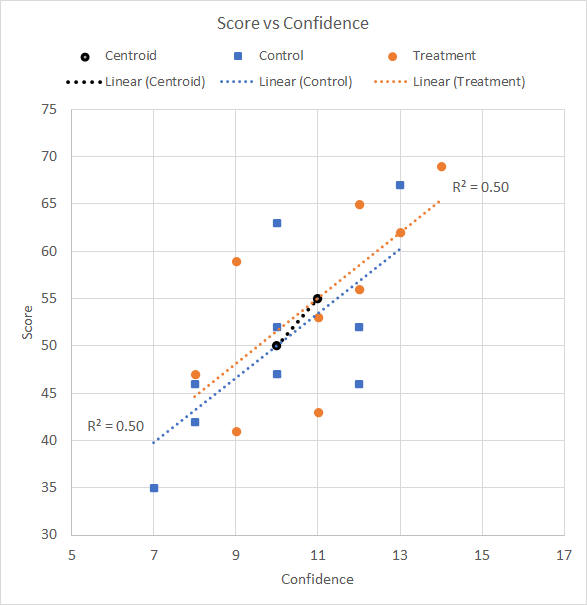
The usual difficulty with a scattergram is seeing what it is telling us.  Here, we (a) add linear trend lines to the Control and Treatment data points, (b) add the R² for the correlation between Confidence and Test score for the Control and Treatment groups, (c) add the Control and Treatment centroids(*), and (d) add the linear trend line of the centroids, to give Figure 2.

* The centroid is the data point for a specific group, Treatment or Control, that comprises the mean Confidence and mean Test score for that group.

Figure 2.  Scattergram of the data of Table 1 with trend lines and centroids added

The R² values helpfully tell us that Confidence and Test score are similarly correlated for the Control and Treatment groups, and that r = 0.71 for each (r = √R²).  With df = 7, the r value is significant with p = 0.03.  The centroids helpfully illustrate the relationship between the group means  Although there is no correlation coefficient relevant to the centroids, the centroid trend line shows a positive relationship which is consistent with the correlation of r = 0.71 for the data of the Control and Treatment groups — that is, higher Confidence is positively associated with a higher Test score.

(§1) Other things being equal, the data should be laid out on axes which are approximately ±3 standard deviations long.  Most graphing software simply fits the data ranges to the axes using whatever aspect ratio for the plot area seemed indicated.  Instead, the plot area should ideally be a square with sides approximately ±3 standard deviations.  A perfect correlation, r = 1, would then be represented by a trend line at 45° running through a centroid in the centre of the plot area.

Multivariate analysis

In SPSS, setting up the dialogue for a multivariate analysis is the same as for a univariate analysis, with the addition that two or more dependent variables are specified instead of just the one.  Table 3 provides the multivariate test for the Table 1 data.

Table 3.  Multivariate test of Table 1 data

Table 3 shows Pillai's Trace as the test statistic;  there are other test statistics, but in this case they give identical results and are omitted.  In general, the four test statistics reported by SPSS are presented in order of their conservative nature.  Pillai's Trace is considered the most conservative — more protective against a Type II error than the other three;  with Roy's Root considered the most liberal, giving a significant results more often than the previous three.

From Table 1, Pillai's Trace = 0.08, equivalent F = 0.62, df = 2 and 15, p = 0.55;  this is most definitely not significant. There is no statistically significant Treatment effect considering Confidence and Test score together.  SPSS also provides the univariate analysis as a "bonus".  Although the omnibus test is not significant and we should not proceed to examining the univariate results, we can enjoy the guilty pleasure of seeing if the elixir perhaps had an effect on Confidence or on Test score considered separately — that is, ignoring the correlation between these two measures.  This is shown in Table 4.

Table 4.  Univariate tests of Table 1 data

Perhaps unsurprisingly, the two univariate tests are not significant, F(1,16) = 1.09, p = 0.31 for Confidence, and F(1,16) = 1.15, p = 0.30, for Test score.  We might wonder briefly why the p value for the multivariate test was higher than those for the univariate tests, imagining they should be similar;  we'll find out why shortly.

But we now need to look at what might have been.

Inconsistent centroid trend

Previously, we noted the centroid trend line showed a positive relationship which was consistent with the positive correlation seen in the data.  Let's take the data of Table 1 and, keeping the effect sizes, imagine our elixir reduced the mean Confidence of the Treatment group by 1, as per Table 5.

Table 5.  Data and descriptive statistics

We see that the Treatment group has a lower mean Confidence than the Control while it has the same higher mean Test score as before.  Just to emphasise the point, the revised effect sizes are shown in Table 6.  They are same absolute size as before, except –0.49 for Confidence rather than +0.49.

Table 6.  Effect sizes

The Confidence and Test score differences are approximately half a standard deviation in size, as before.  How could that change our findings?  Let's look at the scattergram.

Figure 3.  Scattergram of the data of Table 5 with trend lines and centroids added

Figure 3 paints a rather different picture.  Notice that the centroid trend line is the same length, that is, the two centroids are the same distance apart, as we would expect given the effect sizes are the same size;  but here we see that the centroid trend is negative, that is, opposite to the trend we would expect given the positive correlation between Confidence and Test score.  The data of the Control and Treatment groups taken separately both show significant positive correlation where a higher Confidence is positively associated with a higher Test score, but here we see that the elixir seems to have caused a general mean drop in Confidence even while it has given rise to a general increase in mean Test score.  The multivariate test is shown in Table 7.

Table 7.  Multivariate test of Table 5 data

This is significant!  There is a statistically significant Treatment effect considering Confidence and Test score together.  While we ponder the Nobel Prize possibilities for showing how to lower what we will hasten to call over-Confidence and at the same time increase Test scores, the significant multivariate test allows us to examine the elixir effect on Confidence or on Test score considered separately.  This is shown in Table 8.

Table 8.  Univariate tests of Table 5 data

The elixir has no significant effects on Confidence or Test score when these measures are considered separately.  Table 8 is identical to Table 4.  A little thought will explain why — the effect sizes are identical and the standard deviations and correlations are identical.

The multivariate analysis can test and then flag a result that cannot be tested or flagged by univariate tests — whether the Treatment effect is consistent with, or the opposite of, what would be expected given the correlation between the measures.  We hope that, as seasoned researchers, we would have noticed the little detail of how the elixir seemed to reduce Confidence even while seeming to boost Test score, but because the univariate tests were clearly not significant, we certainly could not publish such a non-finding.

Next:  Multivariate Error Oval to visualise the significance of the multivariate difference between two group centroids, and Multivariate Anova part 2.

©2025 Lester Gilbert