Introduction to the analysis of covariance

The analysis of covariance involves the adjustment of the values of a measure of interest according to its relationship with a second measure, sometimes called a nuisance variable. 

We start with a very simple example — an experiment with two groups, Treatment and Control, and the variable of interest, the participants' score on a test of cognitive functioning.  We want to know if a modest dose of caffeine really does boost exam or test performance, or if its effects can be simply explained by its well-known effect on alertness.  As many times in these pages, we recruit 18 of our friends, allocate 9 to the Treatment group and give them a 75 mg dose of caffeine in 250 ml of sweetened brown-coloured water, while the 9 in the Control group are given the same but without any caffeine.  Thirty minutes after their drink they undertake a short test of reaction time (taken as the operational measure of Alertness) and then go on to complete a test of cognitive function.  Alertness is rated on a 20-point scale, 0 = very dozy and 20 = hyper-responsive, and the Test score on cognitive function is a percentage.  The data is shown in Table 1 along with some descriptive statistics.  (The same numerical values feature in the pages on the Multivariate Anova.)

Table 1.  Data and descriptive statistics

We notice that the Treatment group has a higher mean Test score than the Control group, but it also has a higher mean Alertness rating.  We also notice the significant correlation between Alertness and Test score.  We think the correct approach here is to control for the influence of Alertness by statistically adjusting the Test scores, before addressing the question of whether the mean group Test scores are significantly different.  This is the analysis of covariance, Ancova.

Anova refresher

We first remind ourselves of the mechanism of the one-way analysis of variance.  We want to know if there is a significant difference between the mean Test scores of the Treatment and Control groups, which are 55.0 and 50.0 respectively.  Table 2 gives the Anova summary table for our data. 

Table 2.  Anova of Test score.

The Group variance, MS(Group) = 112.5, is the measure of the difference between the Group means of 50 and 55 (§1).  The error variance, MS(Error) = 97.88, is the measure of the variance seen in each cell of 99.5 and 96.25.  If MS(Group) is significantly larger than MS(Error) we conclude that the difference between the means is larger than can be accounted for by random sampling or error variation.  The test is given by the F ratio, the ratio of MS(Group) to MS(Error), which is 1.15, p = 0.30, so not a significant difference.

(§1) We recall that a MS of a factor such as Group is the variance of the means of that factor, multiplied by the number of data items in each mean.  MS(Group) = n * Var(Group means) = 9 * Var(50,55) = 9 * 12.5 = 112.5.

This quick recap is to remind us that there are two values which, when adjusted, affect the test of significance.  One is the value for MS(Group), and it changes if the group means change.  Two is the value for MS(Error), and it changes if the amount of error variation changes.

When we control for the difference in Alertness by statistically adjusting the Test scores, the consequence is to change MS(Group), or MS(Error), or both.  It may be that the mean adjusted Test scores are closer together (the more usual outcome), therefore reducing MS(Group) and tending to reduce or eliminate significance.  It may be that the adjusted Test scores show lower variance (also the more usual outcome), therefore reducing MS(Error) and tending to create or increase significance.  The change to MS(Error) is usually, but not always, good.  The change to MS(Group) is usually, but not always, undesirable.  And the change to both may give an unexpected result.

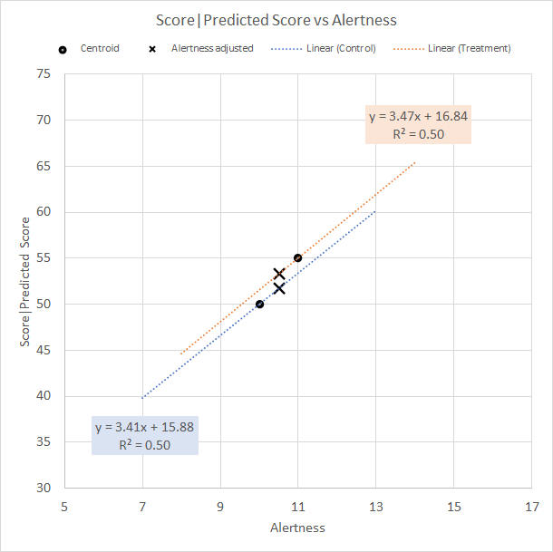
Adjustment mechanism

To adjust for Alertness, we construct a predicted Test score based on the Alertness rating, using the correlation between the two.  The adjustment proceeds in two stages.  The first stage calculates the predicted Test scores in each Group based on the group correlation between Alertness and Test score.  The second stage predicts the Group mean Test scores.  When you read "predicted", you know immediately this is regression, so yes, the Ancova regresses Alertness against Test score.

We pause and wonder why the first stage of prediction does not therefore also give us the second stage.  Well, it would, and does, if there is no mean difference in Alertness between the groups.  The first stage of prediction provides an adjustment to the Test scores using Alertness within each group separately, but does not thereby adjust for any difference in Alertness between the groups.  This must be done in a second stage.

Stage 1

We recall that the square of the correlation coefficient represents the proportion of variance that one variable accounts for in the other variable.  If we know that r = 0.5 between X and Y, for example, we can say that X accounts for 25% of the variance in Y.  If we know that the r between Alertness and Test score is 0.706 on average, we can say that Alertness accounts for 49.9% of the variance in Test score, with 50.1% remaining.  So for stage 1, we can say that MS(Error) for adjusted Test scores, based on their correlation with Alertness, is 50.1% of the MS(Error) of the original unadjusted Test scores.  Yes, conceptually, exactly so.  Computationally, however, a little wrinkle emerges, which is that by making this adjustment we lose a degree of freedom in MS(Adjusted Error).  The computation requires us to calculate SS(Adjusted Error) and df(Adjusted Error), where df(Adjusted Error) = df(Error) – 1 (§2), and then calculate MS = SS/df using the correctly reduced value for df.  For our example data, MS(Error) = 97.88 with df = 16, and MS(Error) for the adjusted Test scores = 52.35 with df = 15.

(§2) The adjustment of one variable by considering its correlation with a second variable, the covariate, can be extended to an adjustment using two, three, or more covariates if we wished.  We lose a degree of freedom for each covariate.

We have completed stage 1 and have the adjusted MS(Error).  Wait....  Why have we not actually calculated predicted Test scores for the 9 participants in the Control group and the 9 in the Treatment group?  Well, we could (and will, later on), but we do not have to.  We can get the result we want, the reduced MS(Error), straight from the average correlation coefficient (§3).

(§3) Conceptually, the reduced MS(Error) is based on the average of the correlations seen in each Group between Test score and Alertness.  For the example data, the correlation in the Control Group is 0.705, and in the Treatment group it is 0.707, giving an average of 0.706.  However, the actual computation does not proceed in this way and gives a (usually slightly) different result.  We may recall how MS(Error) is calculated in the one-way Anova.  We say, conceptually, that it is the average variance seen in the data cells, but we know that it is actually calculated by finding the SS in each cell, adding the cell SS's together, and then dividing by the total of the cell df's.  This is known as pooling the cell error variances, and so we say, more accurately, that MS(Error) is the pooled cell error variance rather than the average cell error variance.  The same holds for our "average" correlation coefficient r.  It is calculated as a pooled r because of the more intricate process involved in calculating within-group or within-subjects r as the pooled cell covariances divided by the pooled cell standard deviations.

Stage 2

This one is fun because it is explained completely visually.  The numbers come later.  What we want is to set an equal mean Alertness rating in each group and have the group mean Test score adjusted according to the correlation between Alertness and Test score.  Figure 1 is a scattergram of the data of Table 1 where Alertness is plotted against Test score.  The trend line of the relationship between Alertness and Test score is given for each group, as is the group centoid (black dot).  We note that a group trend line always passes through the group centroid, and that the slope of the trend line represents the correlation between Alertness and Test score for the group.

What we do is slide a group centroid along the trend line of the group (§4) to give a mean Alertness that is the same as the other group (black cross).  We can then read off the adjusted Test score for that Alertness.

(§4) This is a visual approximation that works well if the group correlations are similar so that the trend lines are similar.  The Excel trend line for a group uses that group's correlation.  The computation of the adjusted Test scores uses the pooled correlation.  If you want an accurate visual reading of the adjusted Test score, you would need to slide the centroid along a trend line that uses the pooled r.  This can be done by imagining (or drawing) a trend line (a) passing through the original centroid, and (b) whose slope is halfway between (the average of) the slopes of the different group trend lines.  See Figure 10 in the Covariance part 2 page on how to plot the average r trend lines by using the predicted Test scores provided by SPSS.

Figure 1.  Group centroids relocated on group trend lines to give equal Alertness means

Inspection of Figure 1 suggests that the adjusted group mean Test score is around 53 for the Treatment group and around 52 for the Control group, and in fact the means are 53.28 and 51.72 (§5) .  From our refresher of the Anova, we recall that we calculate the adjusted MS(Group) for the Test scores as n * Var(Adjusted means) = 9 * Var(53.28,51.72) = 9 * 1.22 = 10.96.

(§5) As reported by the "EMM" (estimated marginal means) button in the SPSS Ancova, see below.  See Figure 10 in the Covariance part 2 page on estimating the predicted mean value by using the trend line equations shown by Excel for the predicted Test scores provided by SPSS.

Ancova in essence

We have calculated our Ancova and lay it out in Table 3 like an Anova summary table.  (There is some rounding error in our calculation of the MS(Group) adjusted Test scores.  Table 3 is what SPSS reports when the data of Table 1 is processed.)

Table 3.  Ancova summary of adjusted Test score.

We compare the Ancova of the adjusted Test scores to the Anova of the unadjusted Test scores and note a couple of points.

The F ratio is much lower and the p value similarly;  after adjusting for Alertness, there is no evidence of a significant difference in mean adjusted Test score between Treatment and Control.

The adjustment reduced both MS(Group) and MS(Error).  The error or sampling variance in the Test scores was reduced from 97.88 to 52.35, so approximately by 50%.  The MS of the difference between the group means was reduced from 112.5 to 10.26, so approximately by 90%.  The actual difference between the group means was reduced from 5.0 (55.0 – 50.0) to 1.56 (53.28 – 51.72), approximately 70%.

It may be helpful to visualise this comparison on a profile plot, as shown in Figure 2.  The SE for the error bars of the adjusted means is given by √MS(Error) / 9 = 2.41.

Figure 2.  Comparison of Anova and Ancova mean Test scores.  Error bars ±1SE

Regression equivalent of Ancova

Let's run a regression analysis which does the equivalent of the Ancova.  We predict Test score from Group membership (§6) and Alertness rating, and inspect the resulting regression coefficients for Group.  That is, we include Alertness in our examination of whether Group membership predicts Test score, and the regression analysis helpfully tells us this when it accounts for the effect of Alertness.  The results are shown in Tables 4, 5, and 6.

(§6) We code Group as a dummy variable, 0 for Control and 1 for Treatment.

Table 4.  Regression summary

Table 5.  Regression Anova summary

Table 6.  Regression coefficients

We compare the Ancova of the adjusted Test scores to the regression of Group membership and Alertness on Test scores and note a couple of points.

Dropping down to Table 6 of coefficients, we recognise the p value for Group as the same as the p value from the Anacova.  (This is relatively comforting, because the regression Anova summary showed a completely different regression p value that we explore shortly.) 

Staying with the Group coefficients, we also recognise the value of B, 1.56, as the difference between the mean adjusted Test scores of the Treatment and Control groups.  We recall the meaning of B in a regression as the change in the variable of interest given a unit change in the other variable.  In this case, the other variable is Alertness, so Test score changes by 1.56 when Alertness changes by 1.  From the descriptives of our data we know that mean Alertness rating for Control is 10.0, and for Treatment is 11.0, so if we want to know the adjusted Test score when Alertness is changed to 10.5 in each group, a change of +0.5 and –0.5, we know to add 1.56 * 0.5 to the Control mean Test score and subtract 1.56 * 0.5 from the Treatment mean Test score.  That gives us the adjusted Test scores for our groups, 51.72 for Control and 53.28 for Treatment, that we saw earlier.  (A little more comfort, because we do not recognise the SE reported for B as 3.53.  Instead, we thought the SE for the adjusted mean Test scores should be something like 2.41.  We'll pick this up later.)

The Beta for Group is shown as 0.08.  We recall the meaning of Beta in a regression as the correlation coefficient between the variable of interest and the predicted Test score when taking the IVs together.  We also see that Beta for Alertness is 0.70 with a p value of 0.002, highly significant.  This is very similar to the correlation coefficient we saw earlier in the descriptives table, r = 0.725, and so we can conclude that it is almost entirely Alertness which contributes to Test scores, while Group membership is shown to separately contribute with a very modest correlation of 0.08, p = 0.66.

Returning to Table 5, we do recognise the values shown for MS(Residual) and df(Residual) in the Regression Anova summary, and they are the same as the values shown in the Ancova for MS(Error) and df(Error).  What we have here is a simple terminological difference.  By convention, a regression analysis lists its error term as "residual".

But why is the Regression entry in Table 5 significant?  The short answer (and there is no long answer) is that the table is reporting the significance of the prediction of Test score from both Group membership and Alertness taken together.  The little give-away is that the degrees of freedom for Regression is 2, indicating there are two predictors here.

There is a very good argument for approaching our research problem — does a dose of caffeine boost test performance or can its effects be explained by its well-known boost on alertness — by a regression analysis.  But we return to a consideration of the more complete Ancova that is reported by a statistical package such as SPSS and the extra value that it provides.

Ancova in (more) detail

Estimated marginal means

SPSS provides an option to request estimated marginal means, which in an Anova is the door through which you access the analysis of main and simple main effects.  In an Ancova, the EMMs are covariate-adjusted, just what is needed to report the Group adjusted means without having to approximate them from the trend line equations or calculate them from the B value in the table of regression coefficients.  These are shown in Table 7.

Table 7.  Estimated marginal means in the Ancova

The EMM table also shows the standard errors for the adjusted means which align better with the values expected from MS(Error) than those that might be taken from the SE of B in the table of regression coefficients.

Ancova summary table

The SPSS Ancova summary table provides the regression analysis in a somewhat disguised form, as shown in Table 8.  Note that the full Ancova table shows even more results, but none relevant to our current discussion.

Table 8.  SPSS Ancova summary table

Here we recognise the main elements of the regression results seen in Tables 4 and 5 earlier.  The Ancova (poorly) labels the main Regression finding as "Corrected", and this has caught out more than one investigator who thought it was their Ancova that was highly significant, rather than the (less relevant) regression.

Predicted Test scores

SPSS can calculate and save the predicted Test scores for our data.  These are the predicted (Alertness-adjusted) Test scores within each of the groups, and are shown in Table 9.

Table 9.  Ancova predicted (Alertness-adjusted) Test scores

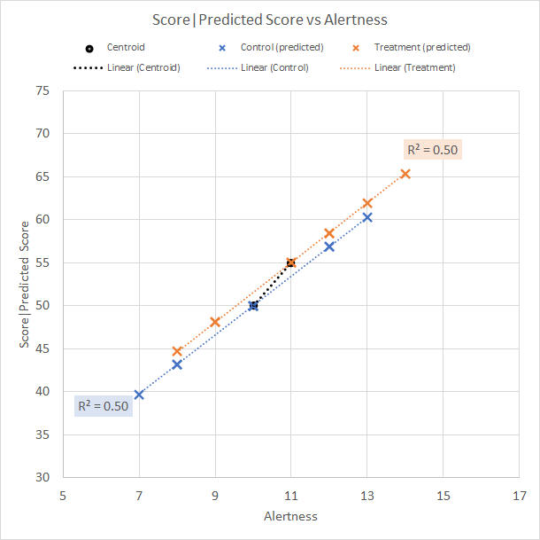
We note that these predicted (adjusted) Test scores retain the same group means, 50.0 for Control, and 55.0 for Treatment.  Figure 3 shows the predicted data points in a scattergram along with the original trend lines for Control and Treatment.

Figure 3.  Scattergram for Table 9 data, predicted (Alertness-adjusted) Test score vs Alertness

The predicted Test scores for a group seem to lie on the group trend line.  This is not the case in general;  instead, they lie on a trend line which uses the average group r for its slope while passing through the centroid of each group.  See Figure 10 in the Covariance part 2 page.

It is also important to note that these predicted Test scores, as such, do not give rise to the Ancova results.  We restate the discussion of Stage 1 to see why not, changing the value of r and adding extra text in [...] to emphasise the point being made:  "If we know that the r between Alertness and Test score is 0.5, we can say that Alertness accounts for 25% of the variance in Test score, with 75% remaining [that is not accounted for by Alertness].  So for stage 1, we can say that MS(Error) for adjusted Test scores, based on their correlation with Alertness, is 75% of the MS(Error) of the original unadjusted Test scores [because it is the error variation NOT accounted for by Alertness which we wish to use]."

So, is there any particular value to routinely saving the predicted values in an Ancova?  Not really, except to plot them in the scattergram and have Excel tell us the adjusted Test scores' prediction equation (trend line equation) for each group (Figure 10 in the Covariance part 2 page).

Next:   Covariance part 2, where we consider a number of data sets, each with a point of interest and see how they turn out on an Ancova, and Covariance part 3 where we consider the possible justification of the use of an Ancova for a data set.

©2025 Lester Gilbert