2D flow simulation (AMYA MY #212)

2D Flow simulation around sail sections

by Lester Gilbert

Sail designers tend to be secretive about the exact sections they use in manufacture, while explicitly claiming the superiority of their product with clarity and force. I entirely lack the dexterity and skill needed to build anything, while being able to construct virtual models and programs without difficulty. I thought it might be interesting to run a variety of plausible sail sections in a virtual wind tunnel to see if there actually were practically distinguishable differences in lift and drag at various wind speeds and angles of attack.

Terminology

Sail sections are described in terms of their chord, amount of maximum draft as a % of chord, and the position of that maximum draft, again as a % of chord. Airfoil sections are generally similarly described in terms of their chord “c”, thickness “t” as a fraction of chord, and position “p” of maximum thickness as a fraction of chord. Although more properly used for wings and sails, the forward part of a sail section or airfoil section is the luff or leading edge and the aft part is the leech or trailing edge. Note that, because wings are “thick” and sails are “thin”, a symmetric wing with t = 0.1, that is, 10% thickness would yield a sail with 5% draft if its upper surface were turned into a sail. Also note that, for the same reason, the visual shape of a wing section is usually dominated by its thickness distribution while the shape of a sail section is completely dominated by its camber distribution.

Section curves

The easiest sail block to make (see Sail blocks analysis for some details of sail making with blocks) would have a circular arc profile, and in order to position maximum draft somewhere other than at 50% of chord it would have a flat aft run, so the short list of plausible section curves begins with “Circular arc” and “Arc with aft run”. An alternative approach is a “Bi-arc” curve which has a smaller radius arc from luff to position of maximum draft and a larger radius arc aft.

NACA comes to mind when thinking about airfoil sections with well-documented characteristics, so the list of candidate sail sections adds the NACA 4-digit camber equation and the NACA 4-digit thickness equation. A NACA 4-digit airfoil section comprises three components, each described by an equation. The first component is the equation for the airfoil nose, and that is a simple circular arc with radius 1.1t².

The second component is the thickness equation, which is also the equation for the upper surface if the airfoil is symmetric. The NACA 4-digit thickness formula is a 4.5^th degree polynomial where maximum thickness occurs at around 30% of chord for a symmetric airfoil.

The third component is the camber line equation, used for asymmetrical airfoils (a symmetric airfoil has zero camber). Here, the amount of camber is added to the amount of thickness to yield the airfoil section shape. The NACA 4-digit camber equation uses two parameters, m = maximum amount of camber as a fraction of chord, and p = position of maximum camber. It effectively constructs a "bi-parabola", with one parabolic curve forward of p, and a second parabolic curve aft of p. For an example of a NACA 4-digit profile, the Cessna 172 has a NACA 2412 wing section, that is, m = 2% maximum camber located at p = 40% of chord with t = 12%.

Deriving a sail section from an equation

Turning an interesting equation into a plausible candidate for a sail section involves a trial and error process. I constructed an Excel spreadsheet to calculate a section using 30 (x, y) data points, and arranged the 4 luff data points to be more closely spaced than the remaining 26 points.

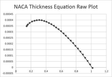
The first step is to guess a range of x values which would provide a section with maximum draft in the desired position, for instance 40%. An example of a plot of the data for the NACA thickness equation is shown in Figure 1 starting at x = 0.14 instead of 0 in order to shift the position of maximum draft aft. The value 0.14 was arrived at after trying 0.13, 0.15, etc. (Note that, by starting at x = 0.14, the curve does not include the nose radius present on an actual NACA profile.)

Figure 1. Raw plot of the NACA thickness equation.

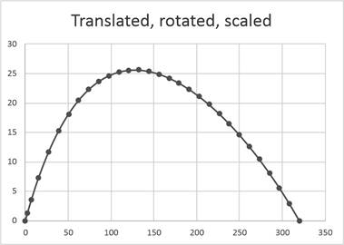
The candidate curve then is translated, rotated, and scaled. Translation moves the data points so that the first point is at (0,0). Rotation then transforms the cartesian points (x,y) to polar coordinates (r, theta) and rotates them so that y₃₀ = 0, that is, the leech lies on the horizontal line through the luff. Scaling returns the polar coordinates to cartesian and adjusts the data points so that x₃₀ = 320, the desired chord, and maximum y = 25.6, the height needed to give the desired 8% draft. The result is illustrated in Figure 2 with exaggerated ordinate.

Figure 2. Plot of the NACA thickness equation from Figure 1 after translation, rotation, and scaling (exaggerated ordinate).

Sail section candidates

In addition to Circular arc, Arc with aft run, Bi-arc, NACA thickness, and NACA camber, other candidate curves for a sail section are Logarithmic Spiral, Archimedean Spiral, Catenary, Parabola, Sine, and Tangent. For all equations, it is the trial and error first step which selects a promising part of the curve for translation, rotation, and scaling to turn it into a section.

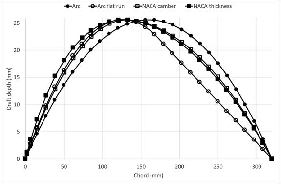
An Excel workbook for each equation was constructed, where each curve of 30 data points was translated, rotated, and scaled to a chord of 320 mm, draft of 8%, and position of maximum draft at 40%, dimensions that might be considered appropriate for the foot of a foresail in a class such as the Marblehead. The sections for Circular arc, Arc with aft run, NACA thickness, and NACA camber are illustrated in Figure 3 with exaggerated ordinate (which is why the circular arc does not look like a circular arc). The other sections mentioned earlier all fall close to or within the profiles shown, some being closer to a circular arc and some being closer to the parabolas of the NACA camber line.

Figure 3. Section curves of 8% maximum camber at 40% of chord plotted with exaggerated ordinate.

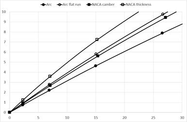
A close-up view of the section entry is given in Figure 4, where the differences in sections are most marked and where it was expected that differences in airflow characteristics would likely be found.

Figure 4. Luff entry for section curves (plotted with exaggerated ordinate).

Generating a simulation model

“Solidworks” is a popular application for 3D design for engineering which has a module for the simulation of structures (finite element analysis, FEA) and flows (computational fluid dynamics, CFD). The simulation module relies on the construction of a mesh of cells which overlay the model under investigation. The behaviour of the fluid or material in a small cell can be relatively easily computed, yielding an overall flow or structural simulation with successive iterations through adjoining cells. This is one way of explaining the essence of FEA and CFD – the quality of its output depends on the quality, coverage, and resolution of the mesh, as does the time taken to run the simulation in silicon.

Running the CFD flow simulations

The CFD simulations were 2D and not 3D. The focus was on the sail section and not on the sail; and since the simulations did not include the effect of a mast, the results are applicable mainly to foresail sections. The global mesh envelope for the virtual wind tunnel comprised a rectangle approximately 3 chord lengths long and 2 chord lengths high, with the section placed in the middle. A higher quality mesh placed a second envelope on the section approximately 2 chord lengths long and one chord length high and generated 4, 8, or 16 sub-cells for every global cell present, while the highest quality mesh placed additional sub-sub-cells around the fluid-body boundary.

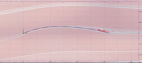
Early results with relatively low-mesh studies could find no differences in the lift and drag performance of the various sail sections, although the qualitative behaviour of the simulations was excellent and plausible, where at various angles of attack and apparent wind speed I could see the formation and dissipation of luff bubbles, upper surface bubbles, and leech vortices. An example of a leech bubble is shown in Figure 5.

Figure 5. Streamlines across a NACA thickness section (8% draft at 40% chord) set at 10° AoA with apparent wind of 5 m/s illustrating a leech bubble (cropped image).

Small differences in lift and drag began to appear with increasing mesh quality, but these differences were sometimes associated with relatively high levels of variation. In addition, at studies beyond stall, very high oscillation in lift and drag was apparent, with effects associated with the periodic formation and shedding of vortices similar to Karman streets. This meant that CL and CD never settled to a constant value and made comparison between different sections difficult. And that is another way of saying that a pinch of salt is needed in drawing conclusions from the data.

In the following simulations, an apparent wind of 5 m/s (around 11 mph) is used, which roughly corresponds to lake-side conditions “at the top of A rig” for an IOM or Marblehead.

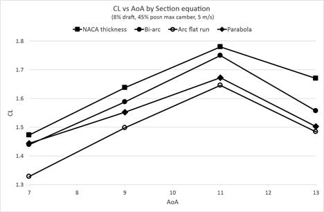
Different sections

Although there were 11 candidate sections in my list, their shapes tended to fall into three groups: like a circular arc, like a parabola, or like the NACA thickness polynomial. Performance did not differ markedly for sections within a group, and so most of the simulations involved sections built from a circular arc, from a parabola, or from the NACA thickness equation.

Figure 6 illustrates the coefficient of lift (CL) for four sail sections run at between 7° and 13° angle of attack (AoA) in a 5 m/s apparent wind. These AoA values were chosen as being just before and just after the section stalls, being the probable use of the section in practice to give maximum drive.

Figure 6. CL for section curves plotted at various AoA.

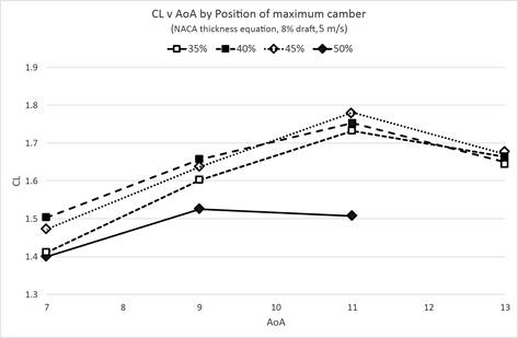
There is some suggestion that the NACA 8458 section has the best performance with CL maximising at around 1.78 just before the stall at 11° AoA, but other data showed it also has close to the highest coefficient of drag (CD) of 0.18 at that point. Inspection of the Lift to Drag (LtoD) curve, a measure of efficiency, suggests little to choose between any of the sections.

Different camber position vs AoA

Figure 7 illustrates CL for the NACA 8xx8 section run at various AoA in a 5 m/s apparent wind, with the xx position of maximum camber set at 35%, 40%, 45%, and 50%.

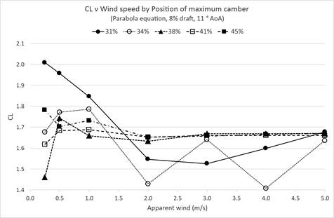
Figure 7. CL for NACA 8xx8 section curve plotted at various AoA.

There seems little to choose between maximum camber set at 40%, 45%, or 50% of chord, though it does seem that setting at 35% does result in poor CL performance with the wind “at the top of the rig”. A L-to-D plot (not shown here) does hint that the usual draft positions of 40% or 45% offer better efficiency than the more extreme 35% or 50% positions.

Different camber position vs apparent wind speed

Figure 8 illustrates CL for a parabola section of various positions of maximum draft run at 11° AoA in a range of apparent winds.

Figure 8. CL for parabola section curve with various positions of maximum draft plotted at various wind speeds.

This plot illustrates the sort of variability seen in runs with lower mesh, and it seems that these runs needed to be at even higher mesh setting in order to reliably separate the different effects of maximum draft position at different wind speeds. While the more extreme forward draft positions of 31% and 34% have low efficiency, in very light winds they show higher CL, in particular for the extremely forward 31% position of maximum camber.

Calibration

A key component of any successful simulation is its validation against previous, physical wind tunnel findings. There is very little published hard data freely available for sails, and so the absolute values in these 2D results, eg a CL of 1.8 for the NACA 8458 at 11° AoA in a 5 m/s wind could be quite wide of the mark. Within a set of runs, however, the relative performance seems plausible.

Simulating a flying shape

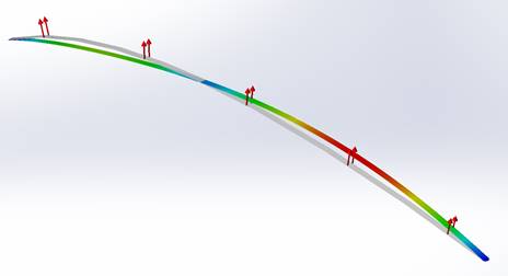
During some discussion of these simulations with Graham Bantock, he wondered what would change if the sail was simulated in “soft” Mylar and hence subject to deformation when flying. An interesting question, since the 2D simulations assume complete rigidity of the section shape. Figure 9 shows the simulated result using FEA of deforming a 3D sail strip of parabolic profile under a constant load along its length equal to the expected lift force from a 5 m/s wind at an angle of attack of 10°. The result is indistinguishable from a circular arc profile.

Figure 9. Deformed Mylar sail strip (exaggerated; shaded resultant force contours) from original parabolic shape (light grey) of 8% draft at 40% chord. Incident wind from left to right in the image.

Conclusions

CFD simulations of different sail sections do show performance differences, but these are subject to a number of caveats. The differences are relatively small; they are highly dependent on the CFD meshing; and they are not calibrated or validated by physical wind tunnel data. On the other hand, within a family of simulations runs, they do show relative differences which can be taken to be indicative.

The shape built into a sail will change as the wind rises. A sail strip constrained at luff and leech adopts a circular arc profile, and this may be the outcome at the sail foot, though sail photos generally show some retention of shape elsewhere.

There is some suggestion that a forward position of maximum draft is effective in drifting to very light winds, and an aft position is more efficient for top of rig conditions.

Acknowedgements

Graham Bantock reviewed an earlier draft and provided comments and corrections. Any remaining errors are exclusively mine.